Backtracking Through Biconnected Components of a Constraint Graph

1 Introduction

Constraint satisfaction problems (CSPs), since their introduction in the early 60's, have flourished in many branches of Artificial Intelligence, and are now used in many "real-life" applications. Since the satisfiability of a CSP is a NP-complete problem, much effort have been devoted to propose faster algorithms and heuristics. Backtrack can be seen as the backbone for those improvements: this algorithm first extends a partial solution by assigning a value to a variable, and undo a previous assignment if no such value can be found.

Backtracking heuristics try to restrict search space, their goal can be to maximize the probability of a "good guess" for the next assignment (variable and value orderings), or to recover more efficiently from a dead-end (backjumping and its variants). Filtering techniques use propagation of some local consistency property ahead of the current partial solution, effectively reducing variable domains; they can be used either in a preprocessing phase, or dynamically during exploration. Structure-driven algorithms emerged from the identification of tractable classes of CSP, such as trees [Mackworth and Freuder, 1985]; they often transform the CSP into one that can be solved in polynomial time [Gottlob et al., 1999].

The algorithm presented, BCC, does not fit easily in this classification. It accepts any preprocessed ordering of the variables, as long as it respects some properties related to the biconnected components of the constraint graph. Then it exploits the underlying tree structure to reduce thrashing dur- Yannic S. Tognetti LIRMM 161, rue Ada 34392 Montpellier, Cedex 5 France E-mail: tognetti@lirmm.fr

ing the backtrack, storing partial solutions and removing permanently some values. Though no kind of local consistency property is used, and no look-ahead is performed, BCC performs well when the graph contains small biconnected components, achieving optimal time complexity in case of a tree.

After basic definitions about CSPs, we present in Sect. 3 the version of Backtrack used as the kernel of BCC. Sect. 4 is devoted to definitions of the variable orderings compatible with BCC. The algorithm is presented in Sect. 5, along with a proof of its soundness and completeness and an evaluation of its worst-case complexity. In Sect. 6, we compare BCC with popular backjumping or filtering techniques, pointing out the orthogonality of these approaches and showing that a mixed algorithm is possible. Finally, we discuss limitations of our algorithm, and suggest a method to overcome them.

2 Definitions and Notations

A binary constraint network a0 over a set of symbols ✁ consists of a set of variables ✂ ✄ ✆ ✞ ✠ ☛ ✌ ✌ ✌ ☛ ✞ ✏ ✒ (denoted ✂ ✔ a0 ✖ ), each ✞ ✘ associated to a finite value domain ✙ ✘ ✛ ✁ , and of a set of constraints. A constraint ✢ ✘ ✣ between two variables ✞ ✘ and ✞ ✣ is a subset of ✙ ✘ ✧ ✙ ✣ . A variable ✞ ✘ is called instantiated when it is assigned a value from its domain. A constraint ✢ ✘ ✣ between two instantiated variables is said satisfied if ✔ value ✔ ✞ ✘ ✖ ☛ value ✔ ✞ ✣ ✖ ✖ ✭ ✢ ✘ ✣ . This test is called a consistency check between ✞ ✘ and ✞ ✣ . A consistent instantiation of a subset ✰ ✛ ✂ ✔ a0 ✖ is an instantiation of all variables in ✰ that satisfies every constraint between variables of ✰ . The CONSTRAINT SATISFACTION PROBLEM (CSP), given a constraint network a0 , asks whether there exists a consistent instantiation of ✂ ✔ a0 ✖ , called a solution of a0 .

Without loss of generality, we can consider that constraints are always defined over two different variables, and that there is at most one constraint (either ✢ ✘ ✣ or ✢ ✣ ✘ ) between two variables. So the constraint graph of a network (associating each variable to a node and connecting two nodes whose variables appear in the same constraint) is a non oriented simple graph without loops. In this paper, we will consider some total order ✷ ✸ on ✂ ✔ a0 ✖ , inducing an orientation of this graph: edges can be seen as oriented from the smallest to the greatest of their ends. According to this orientation, we can define the predecessors ✹ ✺ ✔ ✞ ✖ and the successors ✹ ✾ ✔ ✞ ✖ of a node ✞ . Note that ❀ ✹ ✺ ✔ ✞ ✖ ❀ is the width of ✞ [Freuder, 1982].

3 Back to Backtrack

As the Backtrack algorithm (BT) is the kernel of BCC, we considered as vital to make it as efficient as possible, according to its usual specifications: 1) variables are examined in a fixed, arbitrary ordering; and 2) no information on the CSP is known or propagated ahead of the current variable.

3.1 AlgorithmKernel

Algorithm 1: BackTrack( a0 )

Data : A non empty network ❃ . Result : true if ❃ admits a solution, false otherwise. computeOrder (❄ ); level ❅ 1; failure ❅ false; while ((level ❆ ❇ 0) and (level ❆ ❇ ❈ ✸ ❉ ❃ ❊ ❈ ✾ ✠ )) do currentVariable ❅ ✸ [level]; if (failure) then if (hasMoreValues (currentVariable)) then failure ❅ false; level ❅ nextLevel (currentVariable); else level ❅ previousLevel (currentVariable); else if (getFirstValue (currentVariable)) then level ❅ nextLevel (currentVariable); else failure ❅ true; level ❅ previousLevel (currentVariable); return (level = ❈ ✸ ❉ ❃ ❊ ❈ ✾ ✠ );

As in [Prosser, 1993], BT is presented in its derecursived version: we will later easily control the variable to study after a successful or failed instantiation, without unstacking recursive calls. For the sake of clarity, it is written to solve a decision problem, though a solution could be "read in the variables". This algorithm should consider any variable ordering, so computeOrder only builds the predecessor and successor sets according to the implicit order on the variables, and sorts the predecessors sets (for soundness of partial history). To respect our specifications, if ✞ is the ● th variable according to ✷ ✸ , previousLevel(✞ ) must return ● ❍ ■ and nextLevel( ✞ ) ● ❑ ■ . According to this restriction, our only freedom to improve BT is in the implementation of the functions getFirstValue and hasMoreValues.

3.2 Computing Candidates

Suppose BT has built a consistent instantiation of ✆ ✞ ✠ ☛ ✌ ✌ ✌ ☛ ✞ ✘ ✺ ✠ ✒ . Values that, assigned to ✞ ✘ , would make the instantiation of ✆ ✞ ✠ ☛ ✌ ✌ ✌ ☛ ✞ ✘ ✒ consistent, are the candidates for ✞ ✘ . Then BT is sound and complete if getFirstValue indicates the first candidate, returning false when missing (a leaf dead-end at ✞ ✘ , [Dechter and Frost, 1999]), and successive calls to hasMoreValues iterate through them, returning false when they have all been enumerated (internal dead-end). Testing whether a value is a candidate for ✞ is done in at most width( ✞ ) consistency checks.

The iterative method: The most natural method to implement getFirstValue (resp. hasMoreValues) is to iterate through the domain of ✞ ✘ , halting as soon as a value pass a consistency check with every a80 in ✹ ✺ ✔ ✞ ✘ ✖ , starting at the first domain value (resp. after the last successful value). Both return false when the whole domain has been checked. Though in the worst case, the cost of is ◗ ✔ ❀ ✙ ✘ ❀ width✔ ✞ ✘ ✖ ✖ , values are checked only when needed: this method is good when the CSP is underconstrained or when width( ✞ ✘ ) is small.

The partition refinement method: Suppose ✹ ✺ ✔ ✞ ✘ ✖ ✄ ✆ a80 ✠ ☛ ✌ ✌ ✌ ☛ a80 ❚ ✒ , and note ❲ ❳ the domain ✙ ✘ of ✞ ✘ . Then compute ❲ ✠ ☛ ✌ ✌ ✌ ☛ ❲ ❚ such that ❲ ✣ contains the values of ❲ ✣ ✺ ✠ satisfying the constraint ✢ ✣ ✘ . Then ❲ ❚ is the set of candidates for ✞ ✘ . Though worst case complexity (when constraints are "full") is the same, it is efficient in practice: if ❬ ❭ ❫ ✷ ■ is the constraint tightness of a random network [Smith, 1996], then the expected size of ❲ ✣ ✾ ✠ is ✔ ■ ❍ ❫ ✖ ✧ ❀ ❲ ✣ ❀ ; so the expected time to compute ❲ ❚ is ❀ ✙ ✘ ❀ ❵ ❫ . Though some computed candidates may not be used, this method performs well when constraints tightness and variables width are high. The method hasMoreValues only iterates through this result.

Storing refinement history: A partial history is a trace of the refinements computed in the current branch of the backtrack tree: so having computed ❲ ✠ ✌ ✌ ✌ ❲ ❚ and stored these sets as well as the values of a80 ✣ used to obtain them, if we backtrack up to a80 ❜ and come back again later to ✞ ✘ , we only have to refine domains from ❲ ❜ ✾ ✠ to ❲ ❚ , replacing the previous values. This mechanism is implemented in Alg. 2.

Algorithm 2: getFirstValue( ✞ )

Data : A variable ❡ , belonging to a network ❃ where BT has computed a consistent instantiation of all variables preceding ❡ . We also suppose that ❡ has at least one ancestor. Result : Stores refinement history, and returns true unless the computed set of candidates is empty. last ❅ 1; w ❅ width(❡ ); y ❅ ❢ ❤ [0]; while (last ✐ w and ❥ [last] ❆ ❇ ❦ and usedVal[last] = y.value) do y ❅ ❢ ❤ [last]; last++; while ((last ✐ w) and (❥ [last-1] ❆ ❇ ❦ )) do y ❅ ❢ ❤ [last-1]; usedVal[last] ❅ y.value; ❥ [last] ❅ ❦ ; for (♥ ♦ ❥ [last-1]) do if ((y.value, v) ♦ constraint(y, x)) then ❥ [last] ❅ ❥ [last] a113 a114 v a115 ; last++; success ❅ (last = w+1) and (❥ [last-1] ❆ ❇ ❦ ); if (success) then value ❅ ❥ [last-1][0]; return success;

Each variable ✞ is assigned a field last (denoted, in an OOP style, ✞ .last or simply last when there is no ambiguity), a field value pointing to the current value of ✞ , a vector containing the sorted variables in ✹ ✺ ✔ ✞ ✖ , and two vectors of size width(x)+1: ❲ contains the successive refinements, and usedVal contains the values of the ancestors used for successive refinements of the ❲ ✣ . Note that ❲ [k] contains all values of ❲ [k-1] consistent with the assignment of usedVal[k] to the variable ancestors[k-1]. ❲ [0] is initialized with the domain of ✞ . The partial history mechanism adds the same benefit as Backmarking (BM) [Gaschnig, 1979]. Thoughmorememory expensive (a116 ✔ ❀ ✙ ✘ ❀ ✧ width✔ ✞ ✘ ✖ ✖ space, for each variable ✞ ✘ ) than the usual version of BM, it is more resistant to the jumps forward and backward that will be explicited further in this paper.

4 Variables Orderings Compatible with BCC

Let us now define the particular variable orderings that will be compatible with BCC. Let ✂ ✠ ☛ ✌ ✌ ✌ ☛ ✂ ❚ be ordered subsets of ✂ ✔ a0 ✖ such that ✂ ✔ a0 ✖ ✄ ✇ ❚ ✘ ❇ ✠ ✂ ✘ (their intersection is not necessarily empty), then predset( ✂ ✘ )= ✇ ✘ ✺ ✠ ✣ ❇ ✠ ✂ ✣ . We call an ordering of ✂ ✔ a0 ✖ compatible with this decomposition if, for every subset ✂ ✘ , for every variable ✞ ✭ ✂ ✘ , if ✞ ① ✭ predset ✔ ✂ ✘ ✖ , then ✞ is greater than every variable of predset ✔ ✂ ✘ ✖ . Given such an ordering, the accessor of ✂ ✘ is its smallest element.

4.1 Connected Components

A non empty graph ④ is connected if, for every pair of nodes, there is a walk from one node to the other. A connected component of ④ is a maximum connected subset of ✂ ✔ ④ ✖ .

Now suppose a network a0 whose constraint graph admits ⑤ ⑥ ⑧ connected components, namely ✂ ✠ ☛ ✌ ✌ ✌ ☛ ✂ ❚ . We call a CC-compatible ordering of the variables of a0 an ordering of ✂ ✔ a0 ✖ compatible with some arbitrary ordering of these connected components. Should we launch BT on this network, and should computeOrder store such an ordering, a wellknown kind of thrashing can occur: if BT fails on component ✂ ✘ (i.e. it registers a dead-end at the accessor of ✂ ✘ ), then it will keep on generating every consistent instantiation of the variables in ✂ ✠ ☛ ✌ ✌ ✌ ☛ ✂ ✘ ✺ ✠ to repeat the same failure on ✂ ✘ .

Since the ✂ ✘ represent independent subproblems (a global knowledge on the graph), the usual method is to launch BT on each connected component, stopping the whole process whenever some ✂ ✣ admits no solution. It could also be implemented in a simple way with a slight modification of the function previousLevel: if ✞ is the accessor of a connected component, previousLevel(✞ ) must return 0.

Though very simple, this example illustrates well the method we use later: introduce in the variables ordering some "global" properties of the graph, then use them during backtrack. With a CC-compatible ordering, we benefit from the independence of the sub-problems associated to the connected components; with BCC-compatible orderings, we will benefit from "restricted dependence" between these sub-problems.

4.2 Biconnected Components

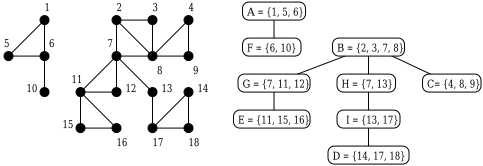
A graph ④ is ⑤ -connected if the removal of any ⑤ ❍ ■ different nodes does not disconnect it. A ⑤ -connected component of ④ is a maximum ⑤ -connected subgraph of ④ . A biconnected component (or bicomponent), is a 2-connected component. Note we consider the complete graph on two vertices biconnected. The graph of bicomponents (obtained by representing each bicomponent as a node, then adding an edge between two components if they share a node) is a forest called the BCC tree of ④ . It is computed in linear time, using two depth-first search (DFS) traversals of ④ [Tarjan, 1972]. Fig. 1 represents a constraint graph and its associated BCC tree.

If we consider the BCC tree as a rooted forest, a natural ordering of its nodes (representing bicomponents) is a total order such that children are greater than their parent. For the BCC tree in Fig. 1, choosing ❷ and ❸ as roots, a DFS could give the order ✆ ❷ ☛ ❹ ☛ ❸ ☛ ④ ☛ ❻ ☛ ❼ ☛ ❽ ☛ ✙ ☛ ❾ ✒ , and a BFS (breadth-first search) ✆ ❷ ☛ ❹ ☛ ❸ ☛ ④ ☛ ❼ ☛ ❾ ☛ ❻ ☛ ❽ ☛ ✙ ✒ . BothDFS and BFS traversals result in a natural ordering.

A BCC-compatible ordering of the variables of a network a0 is an ordering compatible with a natural ordering of its BCC tree (it is also CC-compatible). Such an ordering, if computed by a DFS traversal of the BCC tree, and by a BFS traversal inside the components, would be denoted by a BCC(DFS, BFS) ordering. It can be computed in linear time.

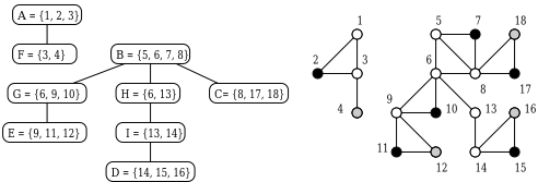
Nodes of the graph in Fig. 2 have been ordered by a BCC(DFS, BFS) ordering. Accessors of a bicomponent have been represented in white. The second variable of a bicomponent is the smallest variable in this component, its accessor excepted. By example, in Fig. 2, 9 is the second variable of the component ✆ ➀ ☛ ➁ ☛ ■ ❬ ✒ . Given a BCC-compatible ordering, the accessor of a variable is defined as the accessor of the smallest (according to the natural ordering) bicomponent in which it belongs. A second variable is always chosen in the neighborhood of its accessor. Tab. 1 gives the accessors determined by the BCC(DFS, BFS) ordering illustrated in Fig. 2.

Suppose a natural ordering of a BCC tree nodes. A leaf variable is the greatest variable appearing in a leaf of the BCC tree. In Fig. 2, leaf variables are coloured in grey. We say that a bicomponent ❾ covers a leaf variable a80 if a80 is the greatest node appearing in the subtree rooted by ❾ (including ❾ itself). Now, we define the compilers of a leaf variable a80 as the accessors of the bicomponents covering a80 . For the ordering in Fig. 2, compilers are: cmp ✔ ➂ ✖ ✄ ✆ ■ ☛ ➅ ✒ , cmp ✔ ■ ⑧ ✖ ✄ ✆ ➀ ☛ ➁ ✒ , cmp ✔ ■ ➀ ✖ ✄ ✆ ➀ ☛ ■ ➅ ☛ ■ ➂ ✒ and cmp ✔ ■ ➇ ✖ ✄ ✆ ➉ ☛ ➇ ✒ .

5 The AlgorithmBCC

The kernel of BCC is BT, as described in Sect. 3. The call to computeOrder orders the variables in a BCC-compatible way, and stores all information on accessors, leaf variables and compilers. This preprocessing takes linear time. We suppose BT is running on a network a0 .

5.1 Theoretical Foundations

Theorem 1 If ✞ is the second variable of some bicomponent, any call to previousLevel(✞ ) can safely (and optimally) return the index of its accessor a80 .

Moreover, no solution of a0 contains the variable a80 instantiated with its current value.

A call to previousLevel(✞ ) means that we have detected some dead-end (either internal or leaf) at variable ✞ . The first part of this theorem asserts that we can backjump right to the accessor of ✞ , without missing any possible solution, and that it could be dangerous to backjump any further (formal definitions about safe and optimal backjumps can be found, by example, in [Dechter and Frost, 1999]). A dead-end found at variable 13 in Fig. 2 would result in a backjump to variable 6. The second part of the theorem means that we can permanently remove the current value of a80 from its domain.

Proof of Theorem 1: The first part is proved by showing that previousLevel( ✞ ) performs a particular case of GraphBased Backjumping (GBBJ) [Dechter, 1990]. The accessor a80 of a second variable ✞ is the only variable in ✹ ✺ ✔ ✞ ✖ . GBBJ performs a safe backjump to the greatest predecessor of ✞ , we have no other choice than a80 . It also adds to a80 a "temporary neighborhood" containing all other predecessors of ✞ (Sect. 6.1). This set being empty, not maintaining it is safe. ➊

Second part relies on the ordering. The following lemma locates the leaf dead-ends responsible for the dead-end at ✞ .

Lemma 1 Let ➋ be the set of variables that registered a dead-end after the last successful instantiation following ✞ . Then variables in ➋ belong to the subtree ➌ of bicomponents rooted by the smallest component containing ✞ (the BCC subtree of ✞ , the accessor of ✞ is also called the accessor of ➌ ).

Sketch of proof: A failure is "propagated upward" in the same bicomponent until a second variable (since variables in the same component, the accessor apart, are numbered consecutively by the compatible ordering). At this point, failure is propagated to the accessor (the backjump in the first part of the theorem), and this accessor belongs to a parent component (a consequence of the natural ordering). ➊

Now suppose there is a solution such that a80 is assigned the value ➍ , and we prove it is absurd. Let us now consider the subnetwork a0 ➎ of a0 , containing all the variables in the the BCC subtree of ✞ , ordered in the same way as in a0 . Let us reduce the domain of a80 in a0 ➎ to ✆ ➍ ✒ . Then a0 ➎ admits a solution, and BT will find the first one for the given ordering. Let us now examine the first leaf dead-end (at variable ✞ ➏ ) that caused to bypass this solution in the BT on a0 (thanks to Lem. 1, it is a variable of a0 ➎ ). Since we had just before a part of the solution of a0 ➎ , the domain of ✞ ➏ has been emptied by a variable outside a0 ➎ (or it would not have been a solution of a0 ➎ ). So there is a constraint between ✞ ➏ and some variable ✞ ➎ ➏ in a biconnected component outside of a0 ➎ : this is absurd, since there would be an elementary cycle ✞ ➏ ☛ ✌ ✌ ✌ ☛ ✞ ☛ a80 ☛ ✌ ✌ ✌ ☛ ➑ ☛ ✌ ✌ ✌ ☛ ✞ ➎ ➏ ☛ ✞ ➏ where ➑ appears in some ancestor of both the component of a80 and the one of ✞ ➏ . Then ✞ ➏ and ✞ ➎ ➏ would be in the same bicomponent. ➊

Since no variable smaller than a80 is responsible for the deadend registered at ✞ , the backjump is optimal. ➒

Theorem 2 We suppose previousLevel has been implemented to match specifications of Th. 1. If ✞ is a leaf variable numbered ● , any call to nextLevel(✞ ), before returning ● ❑ ■ , can mark, for every variable a80 being a compiler of ✞ , that the current value ➍ of a80 has been compiled and that ● ❑ ■ is the forward jump (FJ) for that value (eventually erasing previous FJ for that value).

Thereafter, every time a call to nextLevel should return the index of a second variable ➔ , if the current value ➍ of its accessor → has been compiled, nextLevel can safely (and optimally) return instead the forward jump for ➍ .

Sketch of proof: This is the dual of Th. 1 second part: we had shown that when some failure propagates to the accessor ✞ of a BCC subtree ➌ , then no modification outside ➌ can give a consistent instantiation of ➌ , while keeping ✞ current value. Now, when we have found a consistent instantiation of ➌ , then no modification outside ➌ can make all instantiations of ➌ inconsistent, unless modifying the current value of ✞ . ➒

A call to nextLevel on a leaf means that a whole BCC subtree has been successfully instantiated. In Fig. 2, a call to nextLevel(12) means we have a consistent instanciation of the BCC subtree rooted by the bicomponent ④ covering 12. Before returning 13, this call will store in the accessors of ④ and ❻ their current values ➍ ✔ ➀ ✖ and ➍ ✔ ➁ ✖ , andmark that the FJ for these compiled values is 13. Now we go to 13 and begin to instantiate the subtree containing 6 (already instantiated, and even compiled) and 13, . . . , 16. If there is a dead-end at 13, we should backjump to 6 (see Th. 1), and permanently remove its current value ➍ ✔ ➀ ✖ (we must also remove it from its compiled values). Otherwise, it means we can successfully instantiate this subtree until leaf 16, then make a call to nextLevel. This call updates all information for compilers of 16, and in particular in 6: the FJ for the compiled value ➍ ✔ ➀ ✖ is now 17. Now suppose we have some dead-end at 17. According to Th. 1, we can backjump to 8. Now suppose further failures make us backtrack to 5, that we successfully instantiate, and that we also instantiate 6 with its compiled value. Should a call to nextLevel return 9, it would mean that we found a consistent instantiation of the whole component ✆ ➉ ☛ ➀ ☛ ➣ ☛ ➇ ✒ . Then we know there is a consistent instantiation of ✆ 5,. . . , 16 ✒ , and we can safely jump forward to 17.

5.2 Implementation

Functions previousLevel and nextLevel (Alg. 3, 4) naturally encode the above theorems. nextIndex and previousIndex assume the previous role of nextLevel and previousLevel (returning ● ↕ ■ ).

Algorithm 3: previousLevel( ✞ )

Data : A variable ❡ . Result : The index of the variable to be examined by BCC after a dead-end. if (accessor(❡ ) = x) then return 0; if (isSecondVariable? ( ❡ )) then accessor ❅ accessor(❡ ); val ❅ accessor.value ; for (i = 0; i ✐ width(accessor); i++) do accessor. ❥ [i] ❅ accessor. ❥ [i] ➙ a114 val a115 ; return getIndex (accessor(❡ )); return previousIndex ( ❡ );

Algorithm 4: nextLevel(✞ )

Data ➛ : A variable ❡ . Result : The index of the variable to be examined by BCC after a success. index ❅ nextIndex(❡ ); if (isLeaf?(❡ )) then for ➜ ♦ compilers( ❡ ) do ➜ .compiledValues ❅ ➜ .compiledValues a113 a114 ➜ .valuea115 ; addKey/Value(➜ .FJ, (➜ .value, index)); if (index ❆ ❇ ❈ ✸ ❉ ❃ ❊ ❈ ✾ ✠ ) then nextVariable ❅ V[index]; if (isSecondVariable?(nextVariable)) then accessor ❅ accessor(nextVariable); if (accessor.value ♦ accessor.compiledValues) then index ❅ getKey/Value(accessor.FJ, accessor.value);

return index;

5.3 Worst-Case Complexity

Lemma 2 Using the BCC algorithm, any BCC subtree is entered at most once for each value in its accessor's domain.

Proof: A consequence of Th. 1 and 2. Should we enter a BCC subtree ➌ , either we find a consistent instantiation of ➌ , and the current value for its accessor ✞ is compiled (so every time nextLevel should return the second variable a80 for the smallest bicomponent containing ✞ , it jumps instead to the next subtree); or we have registered some dead-end at a80 (thanks to Lem. 1, this failure came from ➌ ), and the current value for the accessor is permanently removed. ➒

Corollary 1 When a0 is a tree, BCC runs at most in a116 ✔ ➝ ➞ ➟ ✖ , where ➟ ✄ ❀ ✂ ✔ a0 ✖ ❀ and ➝ is the greatest domain size.

Proof: Bicomponents are complete graphs with two nodes (accessor and second variable a80 ). They are entered on a80 , and there will be at most ➝ consistency checks on a80 . There is ➟ bicomponents, each one entered at most ➝ time (Lem. 2). ➒

This result is the same as the one given in [Freuder, 1982], obtained by first achieving arc consistency (a116 ✔ ➝ ➞ ➟ ✖ ), then by a backtrack-free search. Preprocessing required for BCC is linear, and all possible dead-ends can be encountered, but BCC benefits as much from these failures as from successes. This complexity is optimal [Dechter and Pearl, 1988]. Th. 3 extends this result to any constraint graph.

Theorem 3 Let ➟ be the number of bicomponents, ⑤ be the size of the largest one, and ➝ be the size of the largest domain, then BCC runs in the worst case in a116 ✔ ➝ ❚ ➟ ✖ .

Though this worst-case complexity is the same as [Freuder, 1982], BCC should be more efficient in practice: it backtracks along bicomponents instead of generating all their solutions.

6 BCC and Other Algorithms

Though BCC is efficient when the constraint graph contains numerous bicomponents, it is nothing more than a BT inside these components. We study in this section how to improve BCC with some well-known BT add-ons, and point out that BCC reduces the search tree in an original way.

6.1 Backjumping Schemes

To be sound, BCC must perform a very limited form of Backjumping (BJ) (see Th. 1). The natural question is: what if we use more performant backjumps?

Gaschnig's Backjumping (GBJ) [Gaschnig, 1979] is only triggered in case of a leaf dead-end. It jumps back to the first predecessor of ✞ that emptied its domain. This backjump is safe and optimal in case of a leaf dead-end.

Graph-based Backjumping (GBBJ) [Dechter, 1990] is triggered on any dead-end ✞ , and returns its greatest predecessor a80 . Safety is ensured by adding to a80 a temporary set (jumpback set) of predecessors consisting of all the predecessors of ✞ . It is optimal when only graph information is used.

Conflict Directed Backjumping (CDBJ) [Prosser, 1993] integrates GBJ and GBBJ. It backjumps at any dead-end to the greatest variable that removed a value in the domain of ✞ . The jumpback set contains only the predecessors of ✞ that removed some value in ✞ . CDBJ is safe and optimal.

Theorem 4 Let previous(✞ ) be a function implementing a safe Backjump scheme XBJ, always returning the index of a variable a80 belonging to a bicomponent containing ✞ . Then if a80 is the accessor of ✞ , and if no further backjump from a80 will return in the component of ✞ , the current value of a80 can be permanently removed.

The obtained algorithm BCC+XBJ is sound and complete.

Idea of proof: Restrictions enable to paste proof of Th. 1. ➒

Corollary 2 The algorithms BCC+GBJ, BCC+GBBJ and BCC+CDBJ are sound and complete.

Sketch of proof: See that BCC+GBBJ and BCC+CDBJ respect the specifications in Th. 4, and that a backjump on an accessor a80 makes us remove a value only if the jumpback set of a80 only contains its predecessors. Note also that GBJ does not always backjump in the same component (a second variable can backjump to the last element of the parent component, not necessarily the accessor), so BCC specific backjump must be kept to make BCC+GBJ sound and complete. ➒

Finally, we note that these BJ schemes recover more quickly from a failure than BT, but nothing ensures that this failure will not be repeated over and over. BCC's behaviour cannot be obtained by such a BJ mechanism.

6.2 Filtering Techniques

Different levels of arc consistency can be used in algorithms to prune values that become inconsistent ahead of the last instantiated variable. A constraint ✢ ✘ ✣ is said arc-consistent if, ➠ ➡ ✘ ✭ ✙ ✘ , ➢ ➡ ✣ ✭ ✙ ✣ ❵ ✔ ➡ ✘ ☛ ➡ ✣ ✖ ✭ ✢ ✘ ✣ , and conversely.

Maintaining Arc-Consistency (MAC) [Sabin and Freuder, 1994] is believed to be the most efficient general CSP algorithm. This family of algorithms rely on maintaining some kind of arc-consistency ahead of the current variable.

Theorem 5 Let ✞ be the variable currently studied by MAC, and a80 be a variable whose domain was emptied by the AC phase. Let ❾ ✠ ☛ ✌ ✌ ✌ ☛ ❾ ❚ be the bicomponents belonging to the branch of the BCC tree, between the component ❾ ✠ of ✞ and the component ❾ ❚ of a80 . Let ➔ ➞ ☛ ✌ ✌ ✌ ☛ ➔ ❚ be their acessors. Then all values from their domains that were not temporarily removed by the AC phase can be definitively removed by BCC.

Sketch of proof: Consider the accessor ➔ ❚ of the component containing a80 . If AC propagation has emptied the domain of a80 , consider the filtered domain ✙ ➎ ❚ of ➔ ❚ . This failure means that, should we extend our current instantiation of all variables until ✞ with any assignment of ➡ ✭ ✙ ➎ ❚ to ➔ ❚ , this instantiation does not extend to a solution. Thanks to Th. 1, no instantiation of ➔ ❚ with the value ➡ extends to a solution. ➒

Finally, having proven that BCC and MAC combine their effort to produce a good result, we point out that MAC alone cannot replace BCC's efficiency: perhaps MAC will never consider a value that had to be remove by BCC, but should it consider it, nothing will restrain MAC to fail again on it.

7 Conclusion and Future Works

We have presented here a variation on BT called BCC, whose efficiency relies on the number of bicomponents of the constraint graphs. Early tests have shown that, the number of components increasing, BCC alone quickly compensates its inefficiency inside a component and its results are more than a match for other BT improvements. Moreover, we have shown that BCC itself could be added some well-known BT improvements, such as BJ, FC or MAC, effectively combining the best of two worlds. So an improved BCC could be the perfect candidate for networks whose constraint graph contains many bicomponents.

However, we must confess that such constraint graphs are not so common... So, apart from an original theoretical result expressing that a network whose constraint graph is a tree does not need an AC phase nor a backtrack-free search to be solved in a116 ✔ ➝ ➞ ➟ ✖ , what can BCC be used for?

Let a0 be a binary constraint network of size ➟ , and ✞ ✘ and ✞ ✣ be two of its variables. Then we can transform a0 into an equivalent network of ➟ ❍ ■ variables, by fusioning ✞ ✘ and ✞ ✣ into a single variable ✞ ✘ ✣ . The domain of ✞ ✘ ✣ is composed of the pairs of compatible values in the constraint ✢ ✘ ✣ (it is ✙ ✘ ✧ ✙ ✣ when there is no such constraint). Any constraint ✢ ❚ ✘ is then transformed in the followingway: if ✔ ➡ ❚ ☛ ➡ ✘ ✖ ✭ ✢ ❚ ✘ , then all pairs ✔ ➡ ❚ ☛ ✔ ➡ ✘ ☛ ➡ ✖ ✖ such that ✔ ➡ ✘ ☛ ➡ ✖ belongs to the domain of ✞ ✘ ✣ are possible values for the constraint between ✞ ❚ and ✞ ✘ ✣ . The same construction is performed for constraints incident to ✞ ✣ . The obtained network is equivalent, but has now ➟ ❍ ■ variables, and its maximum domain can have now size ➝ ➞ (incident constraints can have size ➝ ➥ ). We can iteratively fusion ⑤ different nodes, obtaining a network of size ➟ ❍ ⑤ ❑ ■ , but where a variable domain can have size ➝ ❚ .

If a constraint graph admits a ⑤ -separator (a set of ⑤ nodes whose removal disconnects the graph), then, by fusioning these ⑤ variables as indicated above, we create at least two bicomponents sharing the obtained variable. Suppose that we can find in some way separators of size ✷ k, the fusion of these separators creating ❫ bicomponents of size ✷ ➦ . Then BCC (without any improvement), will run in time a116 ✔ ➝ ❚ ➧ ❫ ✖ . This decomposition may be quite efficient when ⑤ is small and the separators cut the graph in a non degenerate way, keeping the size of components comparable. This decomposition method (where polynomial cases are obtained when ⑤ and ➦ are both bounded by a constant) is still to be compared to the ones studied in [Gottlob et al., 1999].

To implement and test this decomposition method, we are currently looking for an heuristic that, given an undirected simple graph with weighted edges, find a "small" separator of the graph such that:

1. removal of the separator creates a graph whose greatest connected component is as small as possible;
2. product of the weight on edges that belong to the separator is as small as possible.

The weight on edges will be initialized by the constraint tightness. We believe that networks designed by a human being, who decomposes a problem into subproblems slightly related to each other, will be good candidates for this heuristic.

Acknowledgements

We would like to thanks Christian Bessi`ere for his bibliographical suggestions, Michel Chein and Michel Habib who helped making the concept of "semi-independant subgraphs" evolve into the much more formal one of ⑤ -connected components, as well as the anonymous referees, for their precious comments and advices.