
Fuzzy Conceptual Graphs for Matching Images of Natural Scenes
Proceedings of the Seventeenth International Joint Conference on Artificial Intelligence. Pages 1397-1403.
© 2001 International Joint Conferences on Artificial Intelligence
Abstract
Conceptual graphs are very useful for representing structured knowledge. However, existing formulations of fuzzy conceptual graphs are not suitable for matching images of natural scenes. This paper presents a new variation of fuzzy conceptual graphs that is more suited to image matching. This variant differentiates between a model graph that describes a known scene and an image graph which describes an input image. A new measurement is defined to measure how well a model graph matches an image graph. A fuzzy graph matching algorithm is developed based on error-tolerant subgraph isomorphism. Test results show that the matching algorithm gives very good results for matching images to predefined scene models
- [Kherbeik and Chiaramella, 1995] A. Kherbeik and Y. Chiaramella. Integrating hypermedia and infor- mation retrieval with conceptual graphs. In Proc. Int. Conf. on Hypermedia, Information Retrieval and Multimedia, pages 47-60, 1995.
- [Maher, 1991] P. E. Maher. Conceptual graphs -a frame- work for uncertainty management. In Proc. 10th Annual NAFIPS Conference, pages 106-110, 1991.
- [Mechkour, 1995] M. Mechkour. EMIR2: An extended model for image representation and retrieval. In Proc. Int. Conf. on Databases and Expert Systems Applications (DEXA '95), pages 395-404, 1995.
- [Medasani and Krishnapuram, 1999] S. Medasani and R. Krishnapuram. A fuzzy approach to content-based image retrieval. In Proceedings of the IEEE Conference on Fuzzy Systems, pages 1251-1257, Seoul, 1999.
- [Messmer and Bunke, 1998] B. T. Messmer and H. Bunke. A new algorithm for error-tolerant subgraph isomorphism detection. IEEE Trans. PAMI, 20(5):493-504, 1998.
- [Morton, 1987] S. Morton. Conceptual Graphs and Fuzzi- ness in Artificial Intelligence. PhD thesis, University of Bristol, 1987.
- [Ounis and Pasc ¸a, 1998] I. Ounis and M. Pasc ¸a. RELIEF: Combinig evidences and rapidity into a signle system. In Proc. ACM SIGIR '98, pages 266-274, 1998.
- [Petrakis and Faloutsos, 1997] G. M. Petrakis and C. Falout- sos. Similarity searching in large image databases. IEEE Transactions on Knowledge and Data Engineering, 9(3):435-447, 1997.
- [Sowa, 1984] J. F. Sowa. Conceptual Structures: Informa- tion Processing in Mind and Machine. Addison-Wesley, 1984.
- [Sowa, 1990] J. F. Sowa. Towards the expressive power of natural language. In Proc. 5th Annual Workshop on Con- ceptual Graphs, 1990.
- [Sowa, 1993] J. Sowa. Relating diagrams to logic. In Proc. Int. Conf. on Conceptual Structures (ICCS '93), (LNAI 699), pages 1-35, 1993.
- [Sowa, 2000] J. Sowa. Knowledge Representation: Log- ical, Philosophical, and Computational Foundations.
- [Wuwongse and Manzano, 1993] V. Wuwongse and M. Manzano. Fuzzy conceptual graph. In Proc. Int. Conf. on Conceptual Structures (ICCS '93) (LNAI 699), pages 430-449, 1993.
- [Wuwongse and Tru, 1996] V. Wuwongse and C. H. Tru. To- wards fuzzy conceptual graph programs. In Proc. Int. Conf. on Conceptual Structures (ICCS '96) (LNAI 1115), pages 263-276, 1996.
References were extracted automatically from the PDF and may contain errors.
Full text extracted automatically from the PDF; figures, tables and equations may differ. The PDF is the version of record.
1 Introduction
Conceptual graphs [Sowa, 1984; 1990; 1993; 2000] are expressive for structured knowledge representation and they can be converted to first-order logic expressions. Hence, they are used with theoretical logic-based approaches in applications like hypertext modeling [Kherbeik and Chiaramella, 1995] and image representation and retrieval [Mechkour, 1995; Ounis and Pasc¸a, 1998]. However, in these applications, uncertainty is not represented in the conceptual graphs.
To incorporate uncertainty, Morton [Morton, 1987] extended Sowa's conceptual graph theory to fuzzy conceptual graphs, which include fuzzy referents, fuzzy operations, and fuzzy open and closed worlds. Wuwongse and colleagues [Wuwongse and Manzano, 1993; Wuwongse and Tru, 1996] extended Morton's fuzzy conceptual graphs to incorporate fuzzy conceptual relations. In addition, Maher [Maher, 1991] proposed a similarity measurement for matching simple fuzzy conceptual graphs.
Existing formulations of conceptual graphs are important developments of the theory of fuzzy conceptual graphs. However, they are not suitable for matching uncertain information in images with model scenes. For example, in existing formulations, a concept has only one type. In practice, however, it is very difficult to accurately determine the concept types of the regions in an image. In [Petrakis and Faloutsos, 1997], Attributed Relational Graphs are used for image content representation, and [Medasani and Krishnapuram, 1999] proposed fuzzy matching of these graphs. But, both methods do not handle hierarchies of concept types and of relations.
✄ This research is supported by NUS ARF R-252-000-049-112 and joint NSTB and NUS ARF RP3999903.
This paper presents a new variation of fuzzy conceptual graphs that is more suited to matching images of natural scenes. This variant has several distinct characteristics that distinguish it from existing formulations:
- ☎ It associates a concept with multiple concept types so as to handle the uncertainty of classification.
- ☎ It introduces a new component called relation attribute for capturing concepts such as the ratio between the sizes of two image regions. Separating relation attributes from relations allows two or more correlated relations to share the same attribute explicitly. Relationships between attributes can be represented as well. For example, we can explicitly represent the fact that the ratio between the sizes of two objects is larger than the size ratio of two other objects.
- ☎ It differentiates between model graphs and image graphs. A model graph describes a model of a scene whereas an image graph describes the components and their relationships in an image. As will be described in more details in Section 2, these two types of fuzzy graphs have different characteristics.
- ☎ It defines a similarity measurement between a model graph and an image graph in terms of graph projection. In addition, an algorithm is implemented to compute the similarity based on subgraph isomorphism.
2 Fuzzy Conceptual Graphs
This section first introduces and defines the basic elements of a fuzzy conceptual graph. Next, the degree of match between conceptual graphs is defined and, finally, the graph matching algorithm is described.
2.1 Basic Elements
A fuzzy conceptual graph ✆ ✝ ✟ ✡ ☞ ✡ ✎ ✏ is a directed graph formed from three kinds of components: fuzzy concepts, fuzzy relations, and fuzzy relation attributes. The set ✟ is the set of fuzzy concepts, ☞ the set of fuzzy relations, and ✎ the set of fuzzy relation attributes.
A fuzzy concept ✑ is a 3-tuple ✒ ✓ ✡ ✕ ✡ ✗ ✙ that consists of a set ✓ of concept types ✛ ✜ , a referent ✕ , and a fuzzy membership function ✗ ✝ ✛ ✜ ✏ , ✥ ✦ ✗ ✝ ✛ ✜ ✏ ✦ ✩ for each ✛ ✜ . In [Wuwongse and Manzano, 1993; Wuwongse and Tru, 1996], ✗ ✝ ✛ ✜ ✏ is called the measure assigned to the type ✛ ✜ . In practice, ✗ ✝ ✛ ✜ ✏ can be computed as the confidence of classifying a region as type ✛ ✜ . A crisp concept ✑ can be regarded as a special kind of fuzzy concept whose set ✓ consists of only one concept type ✛ with ✗ ✝ ✛ ✏ ✬ ✩ . For notational convenience, we denote a crisp concept as a 3-tuple of the form ✒ ✛ ✡ ✕ ✡ ✩ ✙ .
A fuzzy relation ✲ is a 2-tuple ✝ ✛ ✡ ✳ ✏ that consists of a crisp relation type ✛ and a fuzziness value ✳ which represents the probability of occurrence of the relation ✲ in the images. A crisp relation is a special kind of fuzzy relation of the form ✝ ✛ ✡ ✩ ✏ , i.e., ✳ ✬ ✩ which means that the relation is not fuzzy.
A fuzzy relation attribute ✹ is a 3-tuple ✒ ✛ ✡ ✕ ✡ ✗ ✙ that consists of a crisp relation attribute type ✛ , a referent ✕ , and a fuzzy membership function ✗ ✝ ✕ ✏ such that ✥ ✦ ✗ ✝ ✕ ✏ ✦ ✩ . A crisp relation attribute is a special kind of fuzzy relation attribute of the form ✒ ✛ ✡ ✕ ✡ ✩ ✙ , where ✗ ✝ ✕ ✏ ✬ ✩ .
The denotation ❂ ✝ ✛ ✏ of type ✛ (concept, relation, or relation attribute type) is the set of all possible individual referents of ✛ . A type ✛ ❃ is a specialization or subtype of type ✛ , denoted ✛ ❃ ✦ ✛ , if ❂ ✝ ✛ ❃ ✏ ❅ ❂ ✝ ✛ ✏ [Sowa, 1984]. The reciprocity holds also. Note that the specialization relationship is reflexive and transitive but not symmetric. The set of concept types together with the specialization relationship forms a finite lattice of concept types. Relation attributes are special kinds of concepts. So, the set of relation attribute types form a sub-lattice in the lattice of concept types. In the same way, the set of relation types forms a finite lattice of relation types.
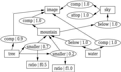
A model graph represents a model of a known scene. In a model, the concept types are known. For example, a mountain-and-lake scene contains sky, mountain, water, tree, etc. (Fig. 1) Therefore, the concepts in a model graph are crisp concepts. However, the relations between the concepts may vary from one image to the next. Moreover, to capture fuzzy linguistics such as "much smaller" and "slightly smaller", the relations and relation attributes have to be fuzzy. For example, the relation ✝ comp ✡ ❈ ✡ ✥ ❊ ● ✏ (represented as ✝ comp ❍ ✥ ❊ ● ✏ in Fig. 1) from ✒ tree✙ to ✒ image✙ indicates that trees appear in 90% of the images of mountain-and-lake scene. The relation ✝ smaller ✡ ❈ ✡ ✥ ❊ ❏ ✏ (represented as ✝ smaller ❍ ✥ ❊ ❏ ✏ in Fig. 1), with attribute ✒ ratio ✡ ❈ ✡ f0.5 ✙ (represented as ✒ ratio ❍ f0.5 ✙ in Fig. 1), from ✒ tree✙ to ✒ mountain✙ indicates that in 70% of the images of mountain-and-lake scene, the area occupied by trees is 50% that of the mountains. The symbol f0.5 denotes a fuzzy membership function that peaks at 0.5. If the ratio ✳ in an input image is not exactly 0.5, then f5.0(✳ ) will be smaller than the maximum value of 1.0.
Several relations can connect the same two concepts in a model graph. Among these relations, those that have the same relation type are regarded as forming a disjunctive group (i.e., OR) of relations (e.g., the "smaller" relation between tree and mountain in Fig. 1). The various disjunctive groups then form a conjunction (i.e., AND) of relations.
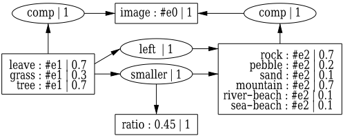
An image graph represents the structure of a particular input image. Due to the inherent uncertainty in the algorithms that classify the image regions, the concepts in an image graph are fuzzy. However, the relations between the regions in an image can be computed exactly. Therefore, the relations and their attributes are not fuzzy. For example, in Fig. 2, due to the ambiguity between leaves texture and grass texture, concept #e1 has a confidence level of 0.7 of being a leave texture or a tree texture, and a lower confidence level of 0.3 of being a grass texture. The rectangular box for #e1 represents the fuzzy concept ✒ ✓ ✡ #e1 ✡ ✗ ✙ where ✓ = ◗ leave, grass, tree ❘ and ✗ (leave) = 0.7, ✗ (grass) = 0.3, and ✗ (tree) = 0.7. The relation ✝ comp ❍ ✩ ✏ from concept #e1 to #e0 is crisp because the region #e1 is a component of the image #e0. Similarly, the relation ✝ smaller ❍ ✩ ✏ and the relation attribute ✒ ratio ❙ ✥ ❊ ❚ ❯ ❍ ✩ ✙ are crisp because the ratio of 0.45 is measured according to the areas of the regions in the image. In summary, a model graph contains crisp concepts, fuzzy relations, and fuzzy relation attributes, while an image graph contains fuzzy concepts, crisp relations, and crisp relation attributes (Table 1).
2.2 Fuzzy GraphMatching
The degree of match between a model graph and an image graph is defined in terms of graph projection [Sowa, 1984] and the degrees of match between their concepts, relations, and relation attributes. The degree of match ❱ between a model concept ✑ ✬ ✒ ✛ ✡ ❈ ✡ ✩ ✙ and an image concept
| element | notation | notation in figure | |
|---|---|---|---|
| model graph | crisp concept fuzzy relation fuzzy relation attribute | ✒ ✛ ✡ ❈ ✡ ✩ ✙ ✝ ✛ ✡ ✳ ✏ ✒ ✛ ✡ ❈ ✡ ✗ ✙ | ✒ ✛ ✙ ✝ ✛ ❍ ✳ ✏ ✒ ✛ ❍ ✗ ✙ |
| image graph | fuzzy concept crisp relation crisp relation attribute | ✒ ✓ ✡ ✕ ✡ ✗ ✙ ✝ ✛ ✡ ✩ ✏ ✒ ✛ ✡ ✕ ✡ ✩ ✙ | ✒ ✛ ✜ ❙ ✕ ❍ ✗ ✝ ✛ ✜ ✏ ✙ ✝ ✛ ❍ ✩ ✏ ✒ ✛ ❙ ✕ ❍ ✩ ✙ |
✑ ❃ ✬ ✒ ✓ ✡ ✕ ✡ ✗ ✙ is defined as
(1)
The degree of match ❱ between a model relation ✲ ✬ ✝ ✛ ✡ ✳ ✏ and an image relation ✲ ❃ ✬ ✝ ✛ ❃ ✡ ✩ ✏ is defined as
The degree of match ❱ between a model relation attribute ✹ ✬ ✒ ✛ ✡ ❈ ✡ ✗ ✙ and an image relation attribute ✹ ❃ ✬ ✒ ✛ ❃ ✡ ✕ ❃ ✡ ✩ ✙ is defined as
A projection ① from a fuzzy graph ✆ ✝ ✟ ✡ ☞ ✡ ✎ ✏ to another fuzzy graph ✆ ❃ ✝ ✟ ❃ ✡ ☞ ❃ ✡ ✎ ❃ ✏ is a mapping such that
- ☎ for each concept ✑ in ✟ , ① ✝ ✑ ✏ is a concept in ✟ ❃ and ❱ ✝ ✑ ✡ ① ✝ ✑ ✏ ✏ ④ ✥ ,
- ☎ for each relation ✲ in ☞ , ① ✝ ✲ ✏ is a relation in ☞ ❃ and ❱ ✝ ✲ ✡ ① ✝ ✲ ✏ ✏ ④ ✥ ,
- ☎ for each relation attribute ✹ in ✎ , ① ✝ ✹ ✏ is a relation attribute in ✎ ❃ and ❱ ✝ ✹ ✡ ① ✝ ✹ ✏ ✏ ④ ✥ ,
- ☎ for any two concepts or relation attributes ⑥ and ✛ related by a relation ✲ in ✆ , ① ✝ ⑥ ✏ and ① ✝ ✛ ✏ are related by ① ✝ ✲ ✏ in ✆ ❃ .
In general, the projection ① ✝ ✆ ✏ may not exist but the projection ① ✝ ⑧ ✏ from a subgraph ⑧ of ✆ may exist. Therefore, the matching problem becomes one of finding the best matching subgraph ⑧ of ✆ that maximizes ❱ ⑩ ✝ ⑧ ✡ ① ✝ ⑧ ✏ ✏ .
Given a projection ① from a subgraph ⑧ ✝ ✟ ✡ ☞ ✡ ✎ ✏ of model graph ✆ to an image graph ✆ ❃ , the degree of match ❱ ⑩ between ⑧ and ① ✝ ⑧ ✏ is defined as
where ❍ ✆ ❍ is the sum of the number of concepts, the number of disjunctive groups of relations, and the sum of the maximum number of relation attributes in each disjunctive group of relation in the model graph ✆ . The second summation in Eq. 4 sums over the conjunctive groups of relations. Note that if ⑧ ✬ ✆ and ❻ ❼ ✬ ❻ ➁ ✬ ❻ ➅ ✬ ✩ , then ❱ ⑩ ✝ ⑧ ✡ ① ✝ ⑧ ✏ ✏ ✬ ❱ ⑩ ✝ ✆ ✡ ① ✝ ✆ ✏ ✏ ✬ ❍ ✆ ❍ ➌ ❍ ✆ ❍ ✬ ✩ . That is, a perfect match yields a matching value of 1. We set ❻ ❼ ✬ ❻ ➁ ✬ ❻ ➅ ✬ ✩ in our test.
2.3 GraphMatching Algorithm
To facilitate the matching process, a graph is first decomposed into a set of arches, each consisting of a source concept ⑥ , a target concept ✛ , a relation ✲ from ⑥ to ✛ , and zero or more relation attributes ✹ ✜ . Thus, arches are actually subgraphs of the model graph or image graph. The match value between a model arch ➎ and an image arch ➎ ❃ is simply the normalized match values of the concepts, relation, and relation attributes of the arches (i.e., Eq. 4).
Our fuzzy graph matching algorithm is a variant of Messmer and Bunke's error-tolerant subgraph isomorphism algorithm [Messmer and Bunke, 1998]. The main differences between these algorithms include the following:
- ☎ In [Messmer and Bunke, 1998], the smallest unit of operation is a vertex. In our algorithm, the smallest unit is an arch.
- ☎ For error-tolerant graph matching, our algorithm needs to consider only deletion of graph vertices. It does not require addition and replacement of vertices and edges, which are supported in [Messmer and Bunke, 1998].
- ☎ Two queues are maintained, one for normal search, and the other one for backtracking to the first-level subgraphs (just below the root). This method improves the quality of the solution found by the algorithm.
The fuzzy graph matching algorithm is as follows:
Convert model graph ✆ to arch set ➏ , image graph ✆ ❃ to arch set ➏ ❃ .
For each pair ✝ ⑧ ✡ ⑧ ❃ ✏ ❦ ➏ ➐ ➏ ❃
Compute ❱ ⑩ ✝ ⑧ ✡ ⑧ ❃ ✏ .
If ❱ ⑩ ✝ ⑧ ✡ ⑧ ❃ ✏ ④ threshold, then insert ✝ ⑧ ✡ ⑧ ❃ ✏ into 1st-level queue ➒ ➓ in decreasing order of ❱ ⑩ ✝ ⑧ ✡ ⑧ ❃ ✏ .
Repeat → times
Empty normal search queue ➒ ➣ . Remove first pair ✝ ⑧ ✡ ⑧ ❃ ✏ from ➒ ➓ and insert into ➒ ➣ . Repeat
Remove first pair ✝ ⑧ ✡ ⑧ ❃ ✏ from ➒ ➣ .
If all arches in ➏ have been considered for connecting to ⑧ , then break out of the inner repeat loop.
For each pair ✝ ➎ ✡ ➎ ❃ ✏ ❦ ➏ ➐ ➏ ❃ such that ❱ ⑩ ✝ ➎ ✡ ➎ ❃ ✏ ④
- 0, ➎ can connect to ⑧ , and ➎ ❃ can connect to ⑧ ❃ Connect ➎ to ⑧ , ➎ ❃ to ⑧ ❃ . Compute ❱ ⑩ ✝ ⑧ ✡ ⑧ ❃ ✏ .
If ❱ ⑩ ✝ ⑧ ✡ ⑧ ❃ ✏ ④ threshold, then insert ✝ ⑧ ✡ ⑧ ❃ ✏ into ➒ ➣ in decreasing order of ❱ ⑩ ✝ ⑧ ✡ ⑧ ❃ ✏ .
Save ✝ ⑧ ✡ ⑧ ❃ ✏ and the match value as a candidate solution.
Return the candidate solution with the highest match value.
The basic idea is to start off with a single arch in the model graph that best matches an arch in the image graph. This pair of arches forms the initial matching model and image subgraphs. Subsequently, other model arches that have matching image arches are added to the matching subgraphs. For model arches that form a disjunctive group, only the best matching model arch is selected. This matching process repeats until all the arches in the model graph have been considered for addition to the matching subgraphs. Then, the matching model and image subgraphs are saved as a candidate solution.
Due to possible ambiguity of the concepts, initial erroneous matches that happen to have large match values may lead the search algorithm down the wrong search paths. So, another queue ➒ ➓ is used to keep the first-level subgraphs. Once a candidate solution is found and saved, the normal search queue ➒ ➣ is emptied and a new search from another firstlevel subgraph is initiated. This method allows the algorithm to escape from local maxima of the solution space. This procedure is repeated → times, and the best solution among them is returned as the final matching result. In the tests reported in Section 3, → is set to 5.
The threshold in the algorithm is used to prune away subgraphs that have poor matching values. This method reduces the amount of searches that need to be considered and helps to improve the efficiency of the algorithm. In the tests, the threshold is set to 0.2.
During the execution of the algorithm, the value ❱ ⑩ ✝ ⑧ ✡ ⑧ ❃ ✏ can be computed incrementally. Let ➙ ✬ ⑧ ➀ ➎ at ✑ , i.e., connecting arch ➎ to model graph ⑧ at the concept ✑ results in the new model graph ➙ . Note that ✑ ❦ ⑧ ✡ ➎ . Similarly, let ➙ ❃ ✬ ⑧ ❃ ➀ ➎ ❃ at ✑ ❃ . Then, ❱ ⑩ ✝ ➙ ✡ ➙ ❃ ✏ can be computed incrementally as follows:
The time complexity of the matching algorithm is ➟ ✝ → ➅ ➠ ➡ ➢ ➠ ✜ ✝ ➤ ➥ ➦ ➠ ❼ ➀ ➤ ➥ ➦ ➠ ➁ ✏ ✏ where ➠ ➢ and ➠ ✜ are the number of model and image arches respectively, → ➅ is the average number of relation attributes per relation, ➠ ❼ is the number of concept types in the concept lattice, ➠ ➁ is the number of relation types in the relation lattice. If each relation has at most one attribute (i.e. → ➅ ✬ ✩ ), then the time complexity reduces to ➟ ✝ ➠ ➡ ➢ ➠ ✜ ✝ ➤ ➥ ➦ ➠ ❼ ➀ ➤ ➥ ➦ ➠ ➁ ✏ ✏ .
3 Test Results
In our current implementation, an input image is segmented using a color and texture segmentation algorithm. The color histogram and Gabor texture features of each region are analyzed to classify the region into several possible classes, and the confidence level for each classification is measured. These measurements are used to generate the image graphs of images by a graph generation program. The model graphs of scene models are generated manually because, at present, we are still in the process of developing a learning algorithm for learning model graphs from example images.
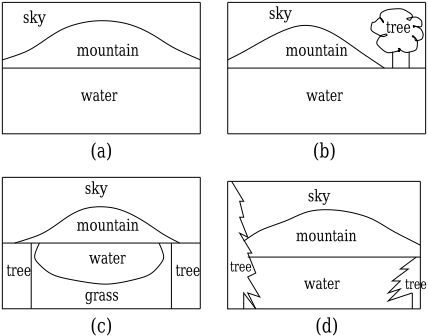
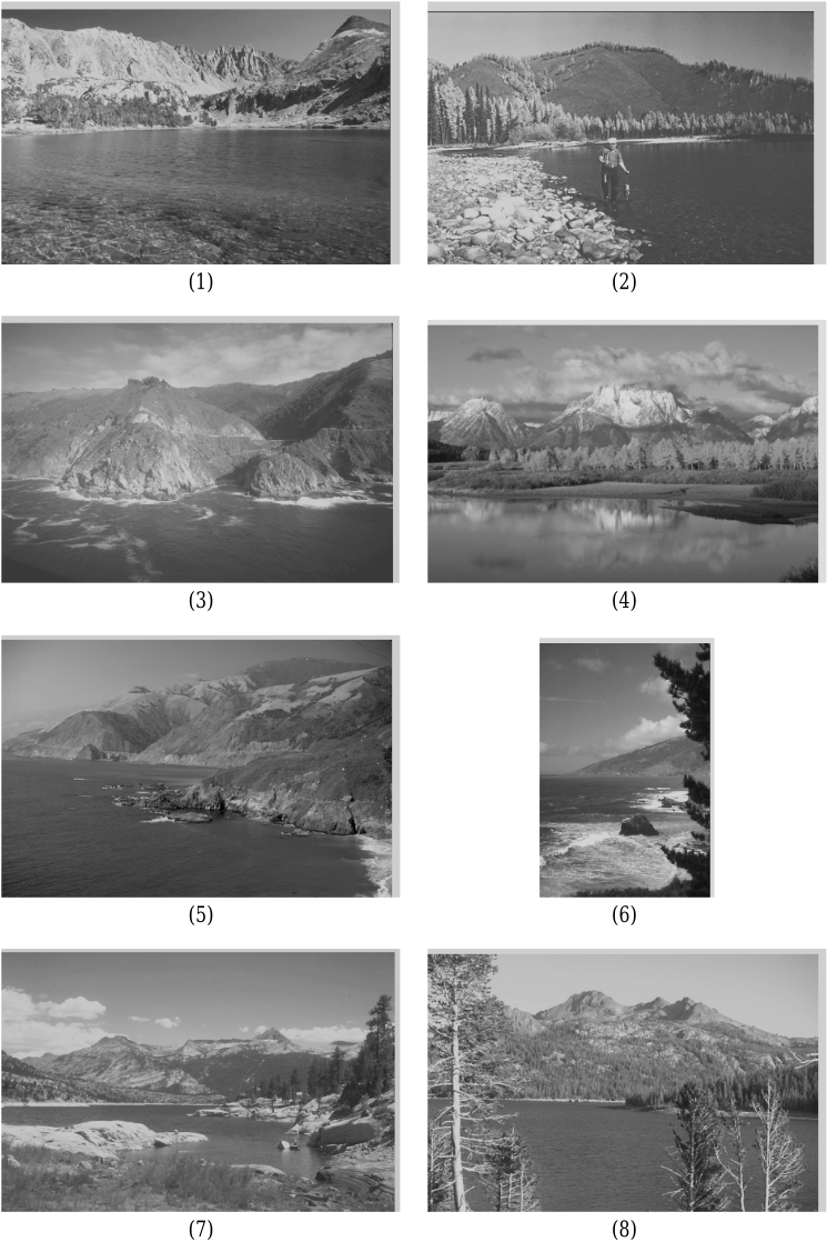
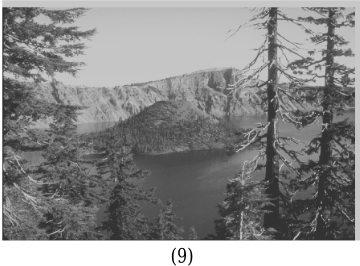
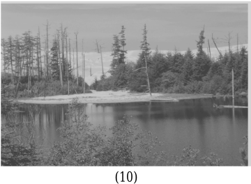
Tests were conducted to match four scene models of different complexity (Fig. 3) with 200 images. A sample of the images are shown in Fig. 4. Table 2 summarizes the test results. Images that match the models well have higher match values than those that match the models poorly. Model ✹ is the simplest among the four models. Most images can fully match model ✹ successfully and thus have high match values. In particular, the first 5 images best match model ✹ and have the highest match values. Model ➨ differs from model ✹ by having a small tree above the water. Therefore, it best matches images 2, 6, and 7.
| model | ||||
|---|---|---|---|---|
| image | ✹ (4,12,0) | ➨ (5,23,6) | ✑ (7,41,12) | ➩ (6,30,9) |
| 1 (4,16,3) | 0.838 | 0.482 | 0.191 | 0.321 |
| 2 (6,29,7) | 0.814 | 0.671 | 0.343 | 0.471 |
| 3 (4,16,3) | 0.814 | 0.444 | 0.177 | 0.367 |
| 4 (7,31,8) | 0.795 | 0.482 | 0.290 | 0.421 |
| 5 (4,18,4) | 0.767 | 0.444 | 0.181 | 0.387 |
| 6 (7,34,10) | 0.686 | 0.666 | 0.354 | 0.485 |
| 7 (8,37,10) | 0.623 | 0.621 | 0.432 | 0.541 |
| 8 (7,35,9) | 0.471 | 0.465 | 0.403 | 0.895 |
| 9 (6,31,9) | 0.519 | 0.371 | 0.313 | 0.638 |
| 10 (8,40,12) | 0.448 | 0.409 | 0.337 | 0.405 |
Model ✑ is the most complex model which has the most number of components. It is used to show that the algorithm can perform partial matching because none of the images can match model ✑ fully. As a result, the images have smaller match values than those for matching the other models. Nevertheless, the ranking of the images is still consistent: images that match model ✑ better have higher match values. In particular, images 7 and 8 match model ✑ best.
Model ➩ is used to illustrate an extreme case in which a very specific model is specified. In this test, model ➩ is created according to image 8. The test results show that image 8 indeed matches model ➩ very well. Image 9 differs a bit from model ➩ in that image 9 has tall trees on both sides of the image whereas model ➩ has tall trees on only one side. Thus, image 9 has a lower match value than image 8. All other images cannot match model ➩ very well and have very small match values.
4 Conclusion
This paper presented a new variant of fuzzy conceptual graphs that is more appropriate than existing formulations for representing and matching input images and model scenes. A new component called relation attribute is introduced into fuzzy conceptual graphs. Moreover, model graphs that describe known scenes are distinguished from image graphs that represent input images. A similarity measure is defined to assess the degree of match between model and image graphs. A graph matching algorithm is developed based on errortolerant subgraph isomorphism algorithm. Experimental tests show that the matching algorithm gives very good results for matching images to scene models.
The fuzzy graphs can be input and modified manually using a graphical user interface. The image graphs of the images that match a model can be displayed by an image retrieval system for explaining how well the image matches the model. We are currently developing a method of learning model graphs given example images of the scenes.
@inproceedings{ijcai2001p184,
  title     = {Fuzzy Conceptual Graphs for Matching Images of Natural Scenes},
  author    = {Mulhem, Philippe and Leow, Wee Kheng and Lee, Yoong Keok},
  booktitle = {Proceedings of the Seventeenth International Joint Conference on
               Artificial Intelligence, {IJCAI-01}},
  publisher = {International Joint Conferences on Artificial Intelligence},
  editor    = {Bernhard Nebel},
  pages     = {1397--1403},
  year      = {2001},
  url       = {https://ijcai.org/proceedings/2001/184},
}
TY - CPAPER TI - Fuzzy Conceptual Graphs for Matching Images of Natural Scenes AU - Mulhem, Philippe AU - Leow, Wee Kheng AU - Lee, Yoong Keok T2 - Proceedings of the Seventeenth International Joint Conference on Artificial Intelligence, IJCAI-01 PB - International Joint Conferences on Artificial Intelligence PY - 2001 SP - 1397 EP - 1403 UR - https://ijcai.org/proceedings/2001/184 ER -Copied
Machine-readable versions of this paper, for tools and AI agents:





