
Sequentially finding the N-Best List in Hidden Markov Models
Proceedings of the Seventeenth International Joint Conference on Artificial Intelligence. Pages 1280-1284.
© 2001 International Joint Conferences on Artificial Intelligence
Abstract
We propose a novel method to obtain the N -best list of hypotheses in hidden Markov model (HMM). We show that the entire information needed to compute the N -best list from the HMM trellis graph is encapsulated in entities that can be computed in a single forward-backward iteration that usually yields the most likely state sequence. The hypotheses list can then be extracted in a sequential manner from these entities without the need to refer back to the original data of the HMM. Furthermore, our approach can yield significant savings of computational time when compared to traditional methods.
- Dawid, A. P. (1992). Applications of a general propagation algorithm for probabilistic expert systems. Statistics and Computing, 2, 25-36.
- Forney, G. (1973). The viterbi algorithm. Proc. IEEE, 61, 268-78.
- Nilsson, D. (1998). An efficient algorithm for finding the m most probable configurations in probabilistic expert systems. Statistics and Computing, 8, 159-73.
- Ostendorf, M. e. a. (1991). Integration of diverse recognition methodologies through reevaluation of n-best sentence hypotheses. In Proceedings, DARPA Speech and Natural language Processing Workshop, pp. 83-7.
- Rabiner, L. (1989). A tutorial on hidden markov models and selected application in speech recognition. Proceedings of the IEEE, 37, (2), 257-86.
- Schwartz, R. and Chow, Y. (1991). A comparison of sev- eral approximate algorithms for finding multiple (n-best) sentence hypotheses. In Proceedings IEEE International Conference on Acoustics, Speech, and Signal Process- ing, pp. 701-4.
- Schwartz, R., Nguyen, L., and Makhoul, J. (1996). Multiple- pass search strategies. In Automatic Speech and Speaker recognition, pp. 429-56. Kluwer Academic Publishers.
- Stolcke, A., Konig, Y., and Weintraub, M. (1997). Explicit word error minimization in n-best list rescoring. Proc. EUROSPEECH, 1, 163-6.
References were extracted automatically from the PDF and may contain errors.
Full text extracted automatically from the PDF; figures, tables and equations may differ. The PDF is the version of record.
1 Introduction
In many tasks of large vocabulary speech recognition it is desirable to find from the HMM graph the N most likely state sequences given the observed acoustic data. The recognizer chooses the utterance hypotheses on the basis of acoustic information and a relatively simple language model. The existence of an N-best list enable us to combine additional knowledge sources such as complicated acoustic and language models into the recognition process [Ostendorf 1991]. Given the additional knowledge sources the list of sentence can be rescored and reordered. Even without additional knowledge sources the N-best paradigm can be used to improve the recognition rate [Stolcke et al. 1997]. In this paper we concentrate on the step of computing the N-best list. The most likely state sequence can be found using a single iteration of the Viterbi algorithm [Rabiner 1989]. A direct generalization of this algorithm can be used to obtain the N best state sequences. The only change is that for each time index t and for each state we have to keep the N best subsequences terminating at this state. However in this generalized Viterbi approach we have to decide in advance on the size of N and we can not change it in the middle of the process. Several modification of this algorithm have been proposed in the last decade. These algorithms are based either on a Viterbi search of a trellis or on A� search [Schwartz and Chow 1991] [Schwartz et al. 1996].
We propose a novel method to obtain the N-best list in HMM. The obtained algorithm is inspired by the divide and conquer algorithm in [Nilsson (1998] for finding the M most likely configurations in probabilistic expert systems. The present algorithm also has the advantage of being an anytime algorithm since we need not in forehand specify the number of N best hypothesis that is wanted. Furthermore, our algorithm can yield significant savings in computational time compared to the traditional Viterbi algorithm.
2 Basic Structure
Consider a HMM with m hidden Markovian random variables X1, . . . , Xm and m observed variables Y1, . . . , Ym such that the distribution of Yt is determined by Xt. Denote X = {X1, . . . ,Xm} and Y = {Y1, . . . , Ym}. Typical values that X and Y can take are denoted x = (x1, . . . , xm) and y = (y1, . . . , ym) respectively. The joint probability function is:
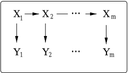
Figure 1: The HMM structure
This paper deals with the following decoding problem: Given observations y1 . . . ym, find the N most likely state sequences of the unobserved state-variables. In other words we want to find the N values of x that maximize the conditional probability function P(x, y) (viewed as a function of x). A single iteration of the forward-backward algorithm [Rabiner 1989] yields the following terms for each time index t:
We shall show that the entire information needed to compute the N-best list is encapsulated in the expressions defined in
(2). In other words, once ft(s) and ft,t+1(s, s′ ) are given, there is no need to refer again to the trellis graph.
As a first example of the usefulness of ft and ft,t+1, we apply them to obtain the most likely state sequence. One can observe that the probability of the most likely state sequence is :
This equality remains the same for each index t = 1, . . . ,m. To find the most likely state sequence ˆx = (ˆx1, . . . , ˆxm), when this is uniquely determined, we note that
However to allow for the possibility that the maximizing state sequence is not unique, it is better to apply the following routine:
3 Introducing the algorithm
Denote the entire ensemble of possible state sequences by X and let the Lth most likely state sequence be denoted
Suppose at some stage in the algorithm that x1 , . . . , xL←1 have been identified. Then xL is found by performing the following steps:
PARTITION PHASE: Here X \ {x1 , . . . , xL←1 } is partitioned into subsets.
CANDIDATE PHASE: For each subset in the above partitioning we compute the probability of its most likely state sequence. These probabilities are referred to as the 'candidates'.
IDENTIFICATION PHASE: The state sequence associated with the highest candidate is identified.
In PARTITION PHASE, there is a large number of possible partitions that one may consider. We seek a partitioning with two properties. Firstly, it must be easy to compute the candidates. Secondly, the number of subsets in the partitioning must be small, since eventually we need to compare the different candidates.
In the successively subsections it is shown how the second and third most likely state sequences are found. In Section 4 the general case is considered.
3.1 The second most likely state sequence
Suppose the most likely state sequence x1 has now been identified. To identify x2 we carry out the following steps.
PARTITION PHASE
Here, X \{x1 } is partitioned into subsets A1, . . . , Am defined
CANDIDATE PHASE
We let ˆ P(Ai) stand for the probability of the most likely state sequence in the subset Ai, i.e.
and use a similar notation for other subsets.
The functions ft,t+1 satisfy that
So, the second most likely state sequence has probability
IDENTIFICATION PHASE
If ˆ P (Ai) = max{ ˆ P(Aj) : j = 1, . . . ,m}, then x2 ∈ Ai, and x2 can be identified by carrying out the following steps:
- � x2j = x1 j for j = 1, . . . , i ← 1.
- � x2 i = argmaxs̸=x1 i fi←1,i(x2 i←1 , s)
- � x2k = argmaxs fk←1,k(x2k←1 , s) for k = i + 1, . . . ,m.
3.2 The third most likely state sequence
The identification of the third most likely state sequence is done by a similar procedure as the case with x2 .
PARTITION PHASE
Here, a partition of X \{x1 , x2} is constructed by refining the above partitioning of X \ {x1}. This is done in the following way.
Suppose x2 ∈ Ai. Then we partitioning Ai \ {x2 } into subsets Bi, . . . , Bm defined by
Thus, the subsets in {Bj : j � i}) and {Aj : j ̸= i}) constitute a partitioning of X \ {x1 , x2}.
CANDIDATE PHASE
As we shall prove in the next section (Theorem 1), the probability ˆ P(Bk) for k � i is a simple function of ˆ P (Ai):
Now, the third most likely state sequence has probability
IDENTIFICATION PHASE
If the third most likely state sequence x3 belongs to one of the subsets Aj (j ̸= i), then it can be identified in a similar way as x2 was identified. On the other hand, if x3 ∈ Bj for some j � i, then
and the sequence x3j , . . . , x3m is now successively identified as follows:
Example To illustrate our algorithm, we consider a simple HMM with 10 hidden variables X1, . . . ,X10, and 10 observed variables Y1, . . . , Y10. Each of the variables are assumed binary with possible states y and n. The initial conditional probability functions associated with the HMM are given in Table 1.
Table 1: The intial probabilities in the HMM
Suppose we obtain 'evidence' of the form
To compute the N-best list given evidence, we initially compute the ft,t+1 functions shown in Table 2. By applying the routine in (3), we can now obtain the most likely state sequence:
with probability P (x1 , y) = .2591 � 10←3 .
For the computation of the second most likely state sequence we proceed as follows. First, we partition the space X \ {x1 } into subsets A1, . . . A10 defined in (4):
Table 2: The ft,t+1 functions (the numbers are multiplied by 103 )
Next, we use (5) to compute the probability of the most likely state sequence in each subsets Ai:
Thus, the second most like state sequence x2 belongs to subset A7, and can be found by carrying out steps (see Section 3.1):
This identifies the second most likely state sequence.
To compute the third most likely state sequence we proceed in a similar manner: First, we partition A7 \ {x2} in subsets of the form in (6):
Then, we compute the probability of the most likely state sequence within each of the subsets Bi. From (7) we immediately obtain ( ˆ P (B7) = 0 since B7 = ∅):
Thus, the third most like state sequence x3 belongs to subset A2, since
and can be found by carrying out the steps described in Section 3.2. This is left to the reader.
Table 3 shows the three most likely state sequences.
| Configuration | Probability (multiplied by 103 ) | |
| x1 = | (n, n, y, y, y, y, y, y, y, y) | P(x1 , y) = .2591 |
| x2 = | (n, n, y, y, y, y, n, n, y, y) | P(x2 , y) = .2185 |
| x3 = | (n, y, y, y, y, y, n, n, y, y) | P(x3 , y) = .1151 |
4 The general algorithm
The general algorithm for computing the N-best list identifies the N most likely state sequences in a sequentialy manner.
Let Xi denote the possible states that the variable Xi can take.
Suppose at some stage in the algorithm that
- � x1 , . . . , xL have been identified;
- � A partitioning, say P L, of X \ {x1 , . . . , xL←1} is given.
- � For each element D in P L, ˆ P(D) is known.
- � xL ∈ D for some element D in the partitioning P L, and D has the following form:
D = {x | x1 = x′1 , . . . , xi←1 = x′i←1 , xi /∈ X ′ i }, (8) where x′1 , . . . , x′i←1 are known states, and X ′ i is a known subset of Xi.
The tasks involved in proving the correcteness of our algorithm consist of:
Partition-phase: Construct a partitioning of D \ {xL};
Candidate-phase: Compute the probability of the most likely state-sequence in each element in the partitioning of D \ {xL};
Identification-phase:
- � Compare the 'new candidates' computed above with the remaining candidates.
- � Identify xL+1 .
These three tasks are described in subsequent subsections.
4.1 Partition phase
Suppose xL ∈ D, where D has the form in (8). For the following analysis it is convenient to write D as
For k = i, . . . , m we define the subsets Dk as
where ¯ Xk is a subset of Xk given by
The reader may easily verify that the subsets Di, . . . , Dm partition D\{xL}. Furthermore, it can be seen that each element Dk has a similar form as that of D.
4.2 Candidate phase
In this section we provide an efficient method to compute the probabilities ˆ P(Dk) (k = i, . . . ,m). The method presented here is similar to the the method in [Nilsson 1998], in that it locally computes the probabilities of all candidates directly from the functions ft,t+1.
A keypoint in proving our main result is that we can write the joint probability function expressed in (1) as
For a proof, the interested reader is referred to [Dawid 1992], where it is shown for more general graphical models, the junction trees.
In addition, we will use that the functions ft,t+1 have the following property, termed max-consistency:
Now we have
Lemma 1 Let E be a subset given by
Then
Proof: The probability ˆ P(E) can be found by instantiating x1 = x�1 , . . . , xi = x�i in (11), and then maximize over the remaining variables. Because of max-consistency (12) this reduces to
which completes the proof. �
Lemma 2 Let D be given as in (9), and suppose
Then for all k = i, . . . , m we have
Proof: Let k � i, and define D′ as
By Lemma 1 it suffices to prove that
Clearly,
since D′ � D. Furthermore, we have that
because xL ∈ D′ and xL = argmaxx∈D P(x, y). The result follows. �
Now we are ready to state the main theorem. It presents a straightforward procedure for finding the probability of each subset Dk (defined in (10)) from the probability ˆ P (D).
Theorem 1 Let D be given as in (9), and suppose
Then for all Dk defined in (10) we have:
Proof: By Lemma 2 we have
Furthermore, since Dk can be written as
Dk = ∪s:s/∈ ¯ Xk {x : x1 = xL1 , . . . , xk←1 = xLk←1 , xk = s}. we have from Lemma 1 that
The result now follows from (13) and (14). �
4.3 Identification phase
Suppose that we are given a subset D of the form
and want to identify the most likely state sequence, say x� , in D. First, one note that
Now the sequence x�i , . . . , x�m is successively found by
4.4 The algorithm
A pseudo code for our N-best list algorithm is given below.
Procedure N-best list:
Step 1 (Identify x1 ):
- Compute the functions ft,t+1;
- Identify the most likely state sequences x1 as shown in Section 3.1;
Step 2 (Identify x2 ):
- �PARTITION PHASE Partition X \ {x1} in subsets A1, . . . ,Am as in (4);
- �CANDIDATE PHASE Compute ˆ P(Ai) as in Section 3.1.
- �IDENTIFICATION PHASE
- Set the Candidate List CL = { ˆ P (Ai)};
- pick the highest candidate, say ˆ P(Ai), in CL;
- identify x2 ∈ Ai as in Section 3.1; .
Step 3 (Identify x3 , . . . , xN )
- �PARTITION PHASE:
- Partition D \ {xL} in subsets Dk, . . . ,Dm as in (10).
- Suppose xL ∈ D;
- �CANDIDATE PHASE: Compute ˆ P(Dk), . . . , ˆ P(Dm) as in Theorem 1.
- �IDENTIFICATION PHASE:
- Augment the Candidate List with the new candidates:
- pick the highest candidate, say ˆ P(D� ), from CL;
- identify xL+1 = argmaxx∈D� P(x, y) as in Section 4.3;
- retract ˆ P(D� ) from the Candidate List: CL := CL \ { ˆ P (D� )}.
END
Accordingly, the probability of the Lth most likely state sequence is either one of the candidates computed in the Lth step of the algorithm or it is one of the candidates computed earlier and still on the Candidate List. The search over all the candidates can be effectively performed in the following way. We can sort the candidates on the Candidate List with their associated subsets. In PARTITION PHASE we split the subsets that contained xL←1 (and hence was at the top of the list) into several subsets. In CANDIDATE PHASE we merge the new candidates into the sorted list according to their probabilities. Now the state sequence xL belongs to the subset at the top of the updated list.
Because the algorithm finds the N-best list sequentially, we need not in forehand specify the number of N best hypothesis that is wanted. In stead, we may chose to find the N most likely hypothesis whose total probability is at least �, where 0 < � � 1.
5 Complexity issues
We would claim that our method can be implemented with lower complexity than traditional methods for finding the Nbest list.
To support this, we would briefly discuss the computational complexity of our method by computing the number of elementary operations needed to perform the various tasks in the algorithm. Let
The operations performed by our algorithm can be divided into three parts
- 1 Computing the functions ft,t+1 and ft defined in (2). and for each L = 1, . . . , N:
- 2 In CANDIDATE PHASE, to compute the candidates as in Theorem 1.
- 3 In IDENTIFICATION PHASE, to compare the candidates on the Candidate List, and identify xL.
Finding the functions in part 1 can be done by less than
In CANDIDATE PHASE, we generate for each step L at most m new candidates. The computation of a candidate takes place via Theorem 1, and can be done with � computaions, i.e. computing all candidates in step L = 1, . . . ,N demands at most
�mN computations.
In IDENTIFICATION PHASE, we compare, in step L at most mL elements (since at most m candidates are generated in each step). If we store the elements in a 2-3 search tree, then the comparisons needed for inserting m new elements and update the search tree is O(mlog(mL)). Doing this for all L = 1, . . . ,N, the total number of comparisons needed is in the order of
Finally, in IDENTIFICATION PHASE, we identify xL as described in Section 4.3, and the number of comparisons needed is no larger than m�. Thus the total number of comparisons cannot exceed
Adding up these terms, we obtain that the whole process of finding x1 , . . . , xN is in the order of
To compare, a straightforward implementation of the Viterbi search as described in [Forney (1973] uses in the order of
We conclude that for large �, our method can yield significant savings of computational time when comparing to traditional Viterbi search.
6 Conclusion
We have presented in this paper a novel method to compute the N most likely state sequences in HMMs. The algorithm has two advantages compared to traditional methods. Firstly it can yield significant gain in computational time. Secondly, it is an anytime algorithm, and thus is also effective in cases where we do not know in advance how many solutions are needed. The main concept is to perform a small preprocessing computation and then we can produce the sequences in an incremental manner. We have concentrated in this paper on applications of the algorithm to speech recognition problems. The proposed algorithm, however, can be applied to many other sources of information that are organized in a hidden Markov model e.g. analysis of DNA sequences and real time robot navigation.
Acknowledgment
This research was supported by DINA (Danish Informatics Network in the Agricultural Sciences), funded by the Danish Research Councils through their PIFT programme.
@inproceedings{ijcai2001p168,
  title     = {Sequentially finding the N-Best List in Hidden Markov Models},
  author    = {Nilsson, Dennis and Goldberger, Jacob},
  booktitle = {Proceedings of the Seventeenth International Joint Conference on
               Artificial Intelligence, {IJCAI-01}},
  publisher = {International Joint Conferences on Artificial Intelligence},
  editor    = {Bernhard Nebel},
  pages     = {1280--1284},
  year      = {2001},
  url       = {https://ijcai.org/proceedings/2001/168},
}
TY - CPAPER TI - Sequentially finding the N-Best List in Hidden Markov Models AU - Nilsson, Dennis AU - Goldberger, Jacob T2 - Proceedings of the Seventeenth International Joint Conference on Artificial Intelligence, IJCAI-01 PB - International Joint Conferences on Artificial Intelligence PY - 2001 SP - 1280 EP - 1284 UR - https://ijcai.org/proceedings/2001/168 ER -Copied
Machine-readable versions of this paper, for tools and AI agents:





