
The Levelwise Version Space Algorithm and its Application to Molecular Fragment Finding
Proceedings of the Seventeenth International Joint Conference on Artificial Intelligence. Pages 853-861.
© 2001 International Joint Conferences on Artificial Intelligence
Abstract
A tight integration of Mitchell’s version space algorithm with Agrawal et al.’s Apriori algorithm is presented. The algorithm can be used to generate patterns that satisfy a variety of constraints on data. Constraints that can be imposed on patterns include the generality relation among patterns and imposing a minimum or a maximum frequency on data sets of interest. The theoretical framework is applied to an important application in chemo-informatics, i.e. that of finding fragments of interest within a given set of compounds. Fragments are linearly connected substructures of compounds. An implementation as well as preliminary experiments within the application are presented.
- [Agrawal et al., 1993] R. Agrawal, T. Imielinski, A. Swami. Mining association rules between sets of items in large databases. In Proceedings of ACM SIGMOD Conference on Management of Data, 1993.
- [Ashby and Patton, 1993] J. Ashby and D. Paton. The Influ- ence of Chemical Structure on the Extent and Sites of Car- cinogenesis for 522 Rodent Carcinogens and 55 Different Human Carcinogen Exposures. Mutation Research, 286:3- 74, 1993.
- [Bayardo, 1998] R. Bayardo. Efficiently mining long pat- terns from databases. In Proceedings of ACM SIGMOD Conference on Management of Data, 1998.
- [Buchanan and Mitchell, 1978] B. Buchanan and T. Mitchell. Model-directed learning of production rules. In Waterman, D. A. and Hayes-Roth, F. (Eds.) Pattern- Directed Inference Systems, Academic Press, New York, 1978.
- [Dehaspe and Toivonen, 1999] L. Dehaspe, H. Toivonen. Disco  very of Frequent Datalog Patterns, in Data Mining and Knowledge Discovery Journal, Vol. 3, 1999.
- [De Raedt, 1998] L. De Raedt. An inductive logic program- ming language for database mining. in Proceedings of the 4th International Conference on Artificial Intelligence and Symbolic Computation, Lecture Notes in Artificial Intelli- gence, Vol. 1476, Springer Verlag, 2000.
- [De Raedt, 2000] L. De Raedt. A Logical Database Mining Query Language. in Proceedings of the 10th Inductive Logic Programming Conference, Lecture Notes in Artifi- cial Intelligence, Vol. 1866, Springer Verlag, 2000.
- [Dong and Li, 1999] G. Dong and J. Li. Efficient mining of emerging patterns : discovering trends and differences. In Proceedings of KDD, ACM, 1999.
- [Gunopulos et al., 1997] D. Gunopulos, H. Mannila, S. Saluja: Discovering All Most Specific Sentences by Ran- domized Algorithms. In Foto N. Afrati, Phokion Kolaitis (Eds.): Database Theory -ICDT '97, 6th International Conference, Lecture Notes in Computer Science 1186, Springer 1997.
- [Han et al., 1999] J. Han, L. V. S. Lakshmanan, and R. T. Ng, Constraint-Based, Multidimensional Data Mining, Com- puter, Vol. 32(8): 46-50, 1999.
- [Han et al., 2000] J. Han, J. Pei, and Y. Yin. Mining fre- quent patterns without candidate generation. In Proceed- ings of ACM SIGMOD Conference on Management of Data , 2000.
- [Hirsh, 1994] H. Hirsh. Generalizing Version Spaces. Ma- chine Learning, Vol. 17(1): 5-46 (1994).
- [Imielinski and Mannila, 1996] T. Imielinski and H. Man- nila. A database perspective on knowledge discovery. Communications of the ACM, 39(11):58-64, 1996.
- [Inokuchi et al., 2000] A. Inokuchi, T. Washio, H. Motoda. An Apriori-based algorithm for mining frequent substruc- tures from graph data. in D. Zighed, J. Komorowski, and J. Zyktow (Eds.) Proceedings of PKDD 2000, Lec- ture Notes in Artificial Intelligence, Vol. 1910, Springer- Verlag, 2000.
- [Kramer and Frank, 2000] S. Kramer and E. Frank. Bottom- Up Propositionalization. Proceedings of the Work-in- Progress Track at the 10th International Conference on Inductive Logic Programming, 156-162, 2000.
- [Kramer and De Raedt, 2001] S. Kramer and L. De Raedt. Feature construction with version spaces for biochemi- cal applications. In Proceedings of the 18th International Conference on Machine Learning, Morgan Kaufmann, 2001.
- [Mannila and Toivonen, 1997] H. Mannila and H. Toivonen, Levelwise search and borders of theories in knowledge dis- covery, Data Mining and Knowledge Discovery, Vol. 1, 1997.
- [Meo et al., 1998] R. Meo, G. Psaila and S. Ceri, An exten- sion to SQL for mining association rules. Data Mining and Knowledge Discovery, Vol. 2, 1998.
- [Mellish, 1990] C. Mellish. The description identification al- gorithm. Artificial Intelligence, 1990.
- [Mitchell, 1982] T. Mitchell. Generalization as Search, Arti- ficial Intelligence, 1980.
- [Ng et al., 1998] R. T. Ng, L. V.S. Lkshmanan, J. Han, and A. Pang. Exploratory mining and pruning optimizations of constrained associations rules. In Proceedings of ACM SIGMOD Conference on Management of Data , 1998.
- [Rosenkranz et al., 1999] H.S. Rosenkranz, A.R. Cunning- ham, Y.P. Zhang, H.G. Clayhamp, O.T. Macina, N.B. Sussmann, S.G. Grant and G. Klopman. Develop- ment, Characterization and Application of Predictive- Toxicology Models. SAR and QSAR in Environmental Re- search, 10:277-298, 1999.
- [Srinivasan et al., 1999] A. Srinivasan, R.D. King and D.W. Bristol. An Assessment of Submissions Made to the Pre- dictive Toxicology Evaluation Challenge. Proc. of IJCAI- 99, 270-275, 1999. IJCAI
References were extracted automatically from the PDF and may contain errors.
Full text extracted automatically from the PDF; figures, tables and equations may differ. The PDF is the version of record.
1 Introduction
Mannila and Toivonen [Mannila and Toivonen, 1997] formulate the general pattern discovery task as follows. Given a database ✂ , a language ✄ for expressing patterns, and a constraint ☎ , find the theory of ✂ with respect to ✄ and ☎ , i.e. ✆ ✝ ✟ ✄ ✡ ✂ ✡ ☎ ✍ ✏ ✒ ✔ ✕ ✄ ✘ ☎ ✟ ✂ ✡ ✔ ✍ ✢ ✤ ✦ ✂ ✩ ✫ ✭ . Viewed in this way ✆ ✝ ✟ ✄ ✡ ✂ ✡ ☎ ✍ contains all sentences within the pattern language considered that make the constraint ☎ true. This formulation of pattern discovery is generic in that it makes abstraction of several specific tasks including the discovery of association rules, frequent patterns, inclusion dependencies, functional dependencies, frequent episodes, ... Also, efficient algorithms for solving these tasks are known (cf. [Mannila and Toivonen, 1997]).
So far the the type of constraint that has been considered is rather simple and typically relies on the frequency of patterns. In the past decade the data mining community spent a lot of effort to efficiently compute patterns having a minimum frequency, such as e.g. Apriori [Agrawal et al., 1993]. In this paper, we will extend this popular data mining model by allowing the user to specify a variety of different constraints on the patterns of interest. The constraints that will be considered involve generality constraints on patterns, e.g. to specify that the patterns of interest are (resp. are not) more general than a specific pattern, as well as frequency constraints. Frequency constraints that are considered either impose a maximum or a minimum frequency on a data set of interest. These constraints can then be combined e.g. in order to discover all patterns that are more general than pattern ✲ , have a minimum frequency ✳ ✴ on the dataset ✶ , and a maximum frequency ✳ ✷ on data set ✹ . The result is a flexible and declarative query language to specify the patterns of interest. From this point of view, the work also fits in the inductive database framework considered by researchers such as [Imielinski and Mannila, 1996; Han et al., 1999; De Raedt, 2000].
The key problem in discovering theories that involve a conjunction of primitive constraints ✺ ✴ ✼ ✽ ✽ ✽ ✼ ✺ ❁ is to efficiently combine the solvers for the primitive constraints ✺ ❃ . It is at this point where Mitchell's version space approach [Mitchell, 1982] is extremely useful. Indeed, each of the primitive constraints results in a version space. Consider e.g. the minimum frequency constraint. As shown by [Mannila and Toivonen, 1997], the minimum frequency constraint results in a space of solutions with the most general pattern ❄ as the only element of the ❅ -set and the ❆ ❇ ❈ boundary as the ❊ -set. Because this property holds for all primitive constraints, the space of solutions of the conjunction of constraints can also be specified as a version space. Moreover, it can ❋ in principle ❋ be computed using Hirsh's version space intersection method [Hirsh, 1994]. However, rather than applying Hirsh's framework, we will employ a tighter integration of version spaces with Apriori.
To demonstrate the relevance of level-wise version spaces, we present an implementation as well as experiments in the domain of molecular fragment finding. Molecular fragments are sequences of linearly connected atoms. They are useful and important for the induction of so-called StructureActivity Relationships (SARs), which are statistical models that relate chemical structure to biological activity. The use of automatically derived fragments in SARs originates from the CASE/MultiCASE systems developed by [Rosenkranz et al., 1999]. With more than 150 published references, the CASE/MultiCASE systems are the most extensively used SAR and predictive toxicology systems. Previous approaches in these areas are based on the "decomposition" of individual compounds: these methods generate all fragments occurring in a given single compound. In this regard, our contribution is a language that enables the formulation of complex queries regarding fragments - users can specify precisely which fragments ● they are interested in. We also implemented an efficient solver to answer queries in this language. Thus, from the algorithmic point of view, it is no longer necessary to process the results of queries post-hoc.
Molecular fragment finding has also been studied within the context of inductive logic programming and knowledge discovery in databases. For instance, Warmr [Dehaspe and Toivonen, 1999] or the approach by Inokuchi et al. [Inokuchi et al., 2000] have been used in this context. Warmr is a system discovering frequently succeeding Datalog queries, and thus is not restricted to fragments. The approach by Inokuchi et al. deals with arbitrary frequent subgraphs, and thus is not restricted to linear fragments. Both approaches differ in that their pattern domain is more expressive, but finding frequent patterns is likely to be more expensive and complex than for linear fragments. Another approach to fragment finding is bottom-up propositionalization [Kramer and Frank, 2000]. All of these approaches handle only minimum frequency thresholds.
In contrast to all these approaches, the presented work allows the specification of all sorts of constraints, for instance regarding generality or frequency. Also, for the first time, one can pose constraints on the maximum frequency of fragments, and not only on the minimum frequency.
Finally, we would like to stress that the integration with version spaces results in a very compact representation of the resulting solutions. Previous methods would typically output all patterns within the version space. This is interesting for understandability reasons and also for further learning with these fragments as features.
The paper is organised as follows : in Section 2, we introduce the molecular fragment finding task and the primitives for querying such fragments, in Section 3, we present the level-wise version space algorithm, in Section 4, we discuss some experiments in molecular fragment finding, and in Section 5, we conclude and touch upon related work.
2 Framework
2.1 Molecular fragment finding
The task to which we will apply our integrated version space - Apriori framework is that of finding all molecular fragments that satisfy a conjunction of constraints ✺ ✴ ✼ ✽ ✽ ✽ ✼ ✺ ❁ .
A molecular fragment is defined as a sequence of linearly connected atoms. For instance, '❏ ❋ ✤ ❋ ✺ ' is a fragment meaning: "an oxygen atom with a single bond to a sulfur atom with a single bond to a carbon atom". In such expressions '✺ ', '✹ ', '✺ ◆ ', etc. denote elements, and ' ❋ ' denotes a single bond, '=' a double bond, '#' a triple bond, and '❖ ' an aromatic bond. As common in the literature, we only consider "heavy" (i.e., non-hydrogen) atoms in this paper.
We assume that the system is given a database of example compounds and that each of the example compounds in the database is described using a 2-D representation. The information given there consists of the elements of the atoms of a molecule and the bond orders (single, double, triple, aromatic). An example compound in such a representation is shown in Fig. 1.
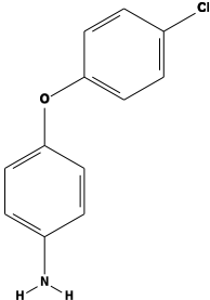
Amolecular fragment ❲ covers an example compound ✫ if and only if ❲ considered as a graph is a subgraph of example ✫ . For instance, fragment '✺ ◆ ❋ ✺ ❖ ✺ ❖ ✺ ❖ ✺ ❋ ❏ ' covers the example compound in Fig. 1.
There are a number of interesting properties of the language of molecular fragments ❪ :
- ❫ fragments in ❪ are partially ordered by the is more general than relation; when fragment ❴ is more general than fragment ✤ we will write ❴ ❵ ✤ ;
- ❫ within this partial order, two syntactically different fragments are equivalent only when they are a reversal of one another; e.g. ' ✺ ❋ ❏ ❋ ✤ ' and ' ✤ ❋ ❏ ❋ ✺ ' denote the same substructure;
- ❫ ❴ ❵ ✤ if and only if ❴ is a subsequence of ✤ or ❴ is a subsequence of the reversal of ✤ ; e.g. '✺ ❋ ❏ ' ❵ '✺ ❋ ❏ ❋ ✤ '.
- ❫ there is a unique maximally general fragment (the empty fragment), which we denote by ❄
- ❫ there is no maximally specific fragment; however, for convenience we add an artificial one to ❪ , which we denote by ❣ .
Note that the representation of molecular fragments is relatively restricted compared to some other representations employed in data mining, such as first-order queries [Dehaspe and Toivonen, 1999] or subgraphs [Inokuchi et al., 2000]. Although fragments are a relatively restricted representation of chemical structure, it is easy for trained chemists to recognize the functional group(s) that a given fragment occurs in. Thus, the interpretation of a fragment reveals more than meets the eye.
2.2 Constraints on fragments
The task addressed in this paper is that of finding the set of all fragments ❲ ✕ ❪ which satisfy a conjunction of primitive constraints ✺ ✴ ✼ ✽ ✽ ✽ ✼ ✺ ❁ . The primitive constraints ✺ ❃ imposed on the unknown target fragments ❲ are :
- ❫ ❲ ❵ ✶ , ✶ ❵ ❲ , ❦ ✟ ❲ ❵ ✶ ✍ and ❦ ✟ ✶ ❵ ❲ ✍ : where ❲ is the unknown target fragment and ✶ is a specific pattern; this type of primitive constraint denotes that ❲ should (not)
be more specific (general) than the specified fragment ✶ ; e.g. the constraint '✺ ❋ ❏ ' ❵ ❲ specifies that ❲ should be more specific than '✺ ❋ ❏ ', i.e. that ❲ should contain ' ✺ ❋ ❏ ' as a subsequence;
- ❫ ❲ ✂ ✫ ☎ ✟ ❲ ✡ ❇ ✍ denotes the frequency of a fragment ❲ on a set of molecules ❇ ; the frequency of a fragment ❲ w.r.t. a dataset ❇ is defined as the number of molecules in ❇ that ❲ covers;
- ❫ ❲ ✂ ✫ ☎ ✟ ❲ ✡ ❇ ✴ ✍ ❵ ✦ , ❲ ✂ ✫ ☎ ✟ ❲ ✡ ❇ ✷ ✍ ♦ ✦ where ✦ is a positive integer and ❇ ✴ and ❇ ✷ are sets of molecules; this constraint denotes that the frequency of ❲ on the dataset ❇ ❃ should be larger than (resp. smaller than) or equal to ✦ ; e.g. the constraint ❲ ✂ ✫ ☎ ✟ ❲ ✡ a114 ❏ ✤ ✍ ♦ a115 a116 a116 denotes that the target fragments ❲ should have a minimum frequency of 100 on the set of molecules a114 ❏ ✤ .
These primitive constraints can now conjunctively be combined in order to declaratively specify the target fragments of interest. Note that the conjunction may specify constraints w.r.t. any number of datasets, e.g. imposing a minimum frequency on a set of active molecules, and a maximum one on a set of inactive ones. E.g. the following constraint: ✟ ' ✺ ❋ ❏ ' ❵ ❲ ✍ ✼ ❦ ✟ ❲ ❵ ' ✺ ❋ ❏ ❋ ✤ ❋ ✺ ❋ ❏ ❋ ✤ ' ✍ ✼ ❲ ✂ ✫ ☎ ✟ ❲ ✡ ② ✺ ✦ ✍ ♦ a115 a116 a116 ✼ ❲ ✂ ✫ ☎ ✟ ❲ ✡ ⑤ ✹ ② ✺ ✦ ✍ ❵ ⑦ ✍ queries for all fragments that include the sequence '✺ ❋ ❏ ', are not a subsequence of ' ✺ ❋ ❏ ❋ ✤ ❋ ✺ ❋ ❏ ❋ ✤ ', have a frequency on ② ✺ ✦ that is larger than 100 and and a frequency on ⑤ ✹ ② ✺ ✦ that is smaller than 5.
3 Solving constraints
In this section, we will discuss how to find the set of all solutions ✤ ❏ ◆ ✟ ✺ ✴ ✼ ✽ ✽ ✽ ✼ ✺ ❁ ✍ in ❪ to a conjunctive constraint ✺ ✴ ✼ ✽ ✽ ✽ ✼ ✺ ❁ .
3.1 The search space
Due to the fact that the primitive constraints ✺ ❃ are independent of one another, it follows that
So, we can find the overall solutions by taking the intersection of the primitive ones.
Secondly, each of the primitive constraints ✺ is monotonic or anti-monotonic w.r.t. generality (cf. [Mannila and Toivonen, 1997]). A constraint ✺ is anti-monotonic (resp. monotonic) w.r.t. generality whenever
(resp. ✟ ❴ ✕ ✤ ❏ ◆ ✟ ✺ ✍ ✍ ❿ ✟ ✤ ✕ ✤ ❏ ◆ ✟ ✺ ✍ ✍ ). The basic anti-monotonic constraints in our framework are: ✟ ❲ ❵ ✶ ✍ ✡ ❲ ✂ ✫ ☎ ✟ ❲ ✡ ❇ ✍ ♦ ✳ , the basic monotonic ones are ✟ ✶ ❵ ❲ ✍ ✡ ❲ ✂ ✫ ☎ ✟ ❲ ✡ ❇ ✍ ❵ ✳ . Furthermore the negation of a monotic constraint is anti-monotonic and vice versa.
Monotonic and anti-monotonic constraints are important because their solution space is bounded by a border. This fact is well-known in both the data mining literature (cf. [Mannila and Toivonen, 1997]), where the borders are often denoted by ❆ ❇ ❈ , as well as the machine learning literature (cf.
[Mitchell, 1982]), where the symbols ❊ and ❅ are typically used.
To define borders, we need the notions of minimal and maximal elements of a set w.r.t. generality. Let ➇ be a set of fragments, then define
We can now define the borders ❊ ✟ ✺ ✍ and ❅ ✟ ✺ ✍ 1 of a primitive constraint ✺ as
Anti-monotonic constraints ✺ will have ❅ ✟ ✺ ✍ ✏ ✒ ❄ ✭ and for proper constraints ❊ ✟ ✺ ✍ ➒ ✏ ✒ ❣ ✭ ; proper monotonic constraints have ❊ ✟ ✺ ✍ ✏ ✒ ❣ ✭ and ❅ ✟ ✺ ✍ ➒ ✏ ✒ ❄ ✭ . Furthermore, as in Mitchell's version space framework we have that
This last property implies that ❊ ✟ ✺ ✍ (resp. ❅ ✟ ✺ ✍ ) are proper borders for anti-monotone (resp. monotone) constraints.
So, we have that the set of solutions ✤ ❏ ◆ ✟ ✺ ❃ ✍ to each primitive constraint is a simple version space completely characterized by ❊ ✟ ✺ ❃ ✍ and ❅ ✟ ✺ ❃ ✍ . Therefore, the set of solutions ✤ ❏ ◆ ✟ ✺ ✴ ✼ ✽ ✽ ✽ ✼ ✺ ❁ ✍ to a conjunctive constraint ✺ ✴ ✼ ✽ ✽ ✽ ✼ ✺ ❁ will also be completely characterized by the corresponding ❊ ✟ ✺ ✴ ✼ ✽ ✽ ✽ ✼ ✺ ❁ ✍ and ❅ ✟ ✺ ✴ ✼ ✽ ✽ ✽ ✼ ✺ ❁ ✍ . At this point there are two issues:
- computing the borders ❊ ✟ ✺ ❃ ✍ and ❅ ✟ ✺ ❃ ✍ for each primitive constraint ✺ ❃
- computing the ❊ ✟ ✺ ✴ ✼ ✽ ✽ ✽ ✼ ✺ ❁ ✍ and ❅ ✟ ✺ ✴ ✼ ✽ ✽ ✽ ✼ ✺ ❁ ✍ given the individual borders ❊ ✟ ✺ ❃ ✍ and ❅ ✟ ✺ ❃ ✍
The first issue could be addressed using (variants of) the common level-wise algorithm for data mining (cf. [Mannila and Toivonen, 1997]). The second one could - in principle - be solved using Hirsh's version space merging algorithm. By now, it is probably clear that we need to integrate the level-wise algorithm with that of version spaces. However, rather than taking a loose coupling of the two approaches (as sketched above) we will provide a tighter integration of the two approaches. As we will show in the experimental section, this will lead to computational advantages.
The integrated algorithm computes the overall border sets incrementally. It initializes the borders ❊ and ❅ with the minimal and maximal elements, and then repeatedly updates for each primitive constraint. To update the borders with regard to a primitive constraint involving generality, it employs Mellish 's description identification algorithm. Mellish's algorithm extends Mitchell's version space algorithm in that it not only allows to process constraints fo the type ❲ ❵ ✶ and ❦ ✟ ❲ ❵ ✶ ✍ 2 but also handles the dual constraints ✶ ❵ ❲ and ❦ ✟ ✶ ❵ ❲ ✍ . Secondly, to update the version space w.r.t. frequency constraints, the integrated algorithm uses a variant of the level-wise algorithm that starts from the given borders rather than from ❄ or ❣ .
1 At this point, we will followMitchell's terminology, because he works with two dual borders (a set of maximally general solutions ↔ and a set of maximally specific ones ↕ ). In data mining, one typically only works with the ↕ -set.
2 The positive and negative examples in concept-learning.
3.2 Mellish's description identification algorithm
In order to formulate Mellish's description identification algorithm, we need to introduce some operations on fragments ❲ ✴ and ❲ ✷ .
- ❫ ❴ ◆ ➙ ✟ ❲ ✴ ✡ ❲ ✷ ✍ ✏ ✳ ➈ ✲ ✒ ❲ ✘ ❲ ✴ ❵ ❲ ➈ ✹ ➑ ❲ ✷ ❵ ❲ ✭ the smallest "merged" fragments
- ❫ ◆ ✩ ➙ ✟ ❲ ✴ ✡ ❲ ✷ ✍ ✏ ✳ ✢ ✹ ✒ ❲ ✘ ❲ ❵ ❲ ✴ ➈ ✹ ➑ ❲ ❵ ❲ ✷ ✭ the largest common subfragments
- ❫ ✳ ❴ ✤ ✟ ❲ ✴ ✡ ❲ ✷ ✍ ✏ ✳ ➈ ✲ ✒ ❲ ✘ ❲ ✴ ❵ ❲ ➈ ✹ ➑ ✹ ❏ ✦ ✟ ❲ ❵ ❲ ✷ ✍ ✭ the smallest fragments more specific than ❲ ✴ but not more general than ❲ ✷
- ❫ ✳ ✤ ❴ ✟ ❲ ✴ ✡ ❲ ✷ ✍ ✏ ✳ ✢ ✹ ✒ ❲ ✘ ❲ ❵ ❲ ✴ ➈ ✹ ➑ ✹ ❏ ✦ ✟ ❲ ✷ ❵ ❲ ✍ ✭ the largest fragments more general than ❲ ✴ but not more specific than ❲ ✷
Notice that these operators may generate more than one fragment; e.g. ◆ ✩ ➙ ✟ ➟ ❏ ✏ ✺ ✏ ✤ ➟ ✡ ➟ ❏ ✏ ✤ ➟ ✍ ✏ ✒ ➟ ❏ ➟ ✡ ➟ ✤ ➟ ✭ . These operations can now be used to instantiate Mellish's algorithm:
❊ := ✒ ❣ ✭ ; ❅ ❼ ✏ ✒ ❄ ✭ ; for all primitive constraint ✺ do case ✺ of ✶ ❵ ❲ : ❊ := ✒ ✤ ✕ ❊ ✘ ✶ ❵ ✤ ✭ ❅ := max ✒ ❴ ◆ ➙ ✘ ❴ ◆ ➙ ✕ ❴ ◆ ➙ ✟ ✶ ✡ ❴ ✍ ➈ ✹ ➑ ❴ ✕ ❅ ➈ ✹ ➑ ➊ ✤ ✕ ❊ ❼ ❴ ◆ ➙ ❵ ✤ ✭ case ✺ of ❲ ❵ ✶ : ❅ := ✒ ❴ ✕ ❅ ✘ ❴ ❵ ✶ ✭ ❊ := min ✒ ◆ ✩ ➙ ✘ ◆ ✩ ➙ ✕ ◆ ✩ ➙ ✟ ✶ ✡ ✤ ✍ ➈ ✹ ➑ ✤ ✕ ❊ ➈ ✹ ➑ ➊ ❴ ✕ ❅ ❼ ❴ ❵ ◆ ✩ ➙ ✭ case ✢ of ❦ ✟ ❲ ❵ ✶ ✍ : ❊ := ✒ ✤ ✕ ❊ ✘ ✹ ❏ ✦ ✟ ✤ ❵ ✶ ✍ ✭ ❅ := max ✒ ✳ ✘ ➊ ❴ ✕ ❅ ❼ ✳ ✕ ✳ ❴ ✤ ✟ ❴ ✡ ✶ ✍ ➈ ✹ ➑ ➊ ✤ ✕ ❊ ❼ ✳ ❵ ✤ ✭ case ✢ of ❦ ✟ ✶ ❵ ❲ ✍ : ❅ := ✒ ❴ ✕ ❅ ✘ ✹ ❏ ✦ ✟ ✶ ❵ ❴ ✍ ✭ ❊ := min ✒ ✳ ✘ ➊ ✤ ✕ ❊ ❼ ✳ ✕ ✳ ✤ ❴ ✟ ✤ ✡ ✶ ✍ ➈ ✹ ➑ ➊ ❴ ✕ ❅ ❼ ❴ ❵ ✳ ✭3.3 Variants of the level-wise algorithm
The algorithms outlined below employ refinement operators.
- ❫ A refinement operator ➤ ➥ ✟ ❲ ✍ ✏ ✳ ➈ ✲ ✒ ❲ ➟ ✕ ❪ ✘ ❲ ➧ ❲ ➟ ✭ , i.e. extending a fragment by one atom.
- ❫ A generalization operator ➤ ➨ ✟ a114 ✍ ✏ ✳ ✢ ✹ ✒ ❲ ➟ ✕ ❪ ✘ ❲ ➟ ➧ a114 ✭ , i.e. removing one atom from one side of a fragment.
To deal with the frequency constraints ✺ , we may employ the following generalization of the level-wise algorithm. This is the downwards version.
Let ✺ be a constraint of type ❲ ✂ ✫ ☎ ✟ ❲ ✡ ❇ ✍ ♦ ✳ ➭ ➯ ❼ ✏ ❅ ; ✢ ❼ ✏ a116 while ➭ ❃ ➒ ✏ ➵ do ➇ ❃ ❼ ✏ ✒ ✶ ✘ ✶ ✕ ➭ ❃ and p satisfies constraint ✺ ✭ ⑤ ❃ ❼ ✏ ➭ ❃ ❋ ➇ ❃ the set of infrequent fragments considered ➭ ❃ ❈ ✴ ❼ ✏ ✒ ✶ ✘ ➊ ☎ ✕ ➭ ❃ ❼ ✶ ✕ ➤ ➥ ✟ ☎ ✍ ➈ ✹ ➑ ➊ ✤ ✕ ❊ ❼ ✶ ❵ ✤ ➈ ✹ ➑ ➤ ➨ ✟ ✶ ✍ ❹ ✟ ➸ ➺ ⑤ ➺ ✍ ✏ ➵ ✭ ✢ ❼ ✏ ✢ ➻ a115endwhile❅ ❼ ✏ ➇ ➯ ❊ ❼ ✏ ✳ ✢ ✹ ✟ ➸ ➺ ➇ ➺ ✍To explain the algorithm, let us first consider the case where ❊ ✏ ✒ ❣ ✭ and ❅ ✏ ✒ ❄ ✭ . In this case, the above algorithmwill behave roughly as the level-wise algorithm. The ➭ ❃ will then contain only fragments of size ✢ and the algorithm will keep track of the set of frequent fragments ➇ ❃ as well as the infrequent ones. The algorithmwill then repeatedly compute a set of candidate refinements ➭ ❃ ❈ ✴ , delete those fragments that cannot be frequent by looking at the frequency of its generalizations, and evaluate the resulting possibly frequent fragments on the database. This process continues until ➭ ❃ becomes empty.
The basic modifications to the level-wise algorithm that we made are concerned with the fact that we need not consider any fragment that is not in the already computed version space (i.e. any element not between an element of the ❅ and the ❊ set). Secondly, we have to compute the updated ❊ set, which should contain all frequent fragments whose refinements are all infrequent.
Finding the updated ❅ and ❊ sets can also be realized in the dual manner. In this case, one will initialize ➭ ➯ with the elements of ❊ and proceed otherwise completely dual.
The resulting upwards algorithm is shown below:
Let ✺ be a constraint of type ❲ ✂ ✫ ☎ ✟ ❲ ✡ ❇ ✍ ♦ ✳ ➭ ➯ ❼ ✏ ❊ ; ✢ ❼ ✏ a116 while ➭ ❃ ➒ ✏ ➵ do ➇ ❃ ❼ ✏ ✒ ✶ ✘ ✶ ✕ ➭ ❃ and p satisfies constraint ✺ ✭ ⑤ ❃ ❼ ✏ ➭ ❃ ❋ ➇ ❃ the set of infrequent fragments considered ➭ ❃ ❈ ✴ ❼ ✏ ✒ ✶ ✘ ➊ ☎ ✕ ➭ ❃ ❼ ✶ ✕ ➤ ➨ ✟ ☎ ✍ ➈ ✹ ➑ ➊ ❴ ✕ ❅ ❼ ❴ ❵ ✶ ➈ ✹ ➑ ➤ ➥ ✟ ✶ ✍ ❹ ✟ ➸ ➺ ➇ ➺ ✍ ✏ ➵ ✭ ✢ ❼ ✏ ✢ ➻ a115 endwhile ❅ ❼ ✏ ✒ ❴ ✕ ❅ ✘ ❴ ✤ ➈ ✦ ✢ ✤ ❲ ✢ ✫ ✤ ✺ ✭ ❊ ❼ ✏ ✳ ✢ ✹ ✟ ➸ ➺ ➇ ➺ ✍Whether the top down or bottom up version works more efficiently is likely to depend on the application and query under consideration. At this point it remains an open question as to when which strategy works more efficiently.
Finally, it is also possible to modify the above algorithms (exploiting the dualities) in order to handle monotonic frequency constraint of the form ❲ ✂ ✫ ☎ ✟ ❲ ✡ ❇ ✍ ❵ ✳ . In this case, one can use the following algorithm (or its dual):
Let ✺ be a constraint of type ❲ ✂ ✫ ☎ ✟ ❲ ✡ ❇ ✍ ❵ ✳ ➭ ➯ ❼ ✏ ❅ ; ✢ ❼ ✏ a116 while ➭ ❃ ➒ ✏ ➵ do ⑤ ❃ ❼ ✏ ✒ ✶ ✘ ✶ ✕ ➭ ❃ and p satisfies constraint ✺ ✭ ➇ ❃ ❼ ✏ ➭ ❃ ❋ ⑤ ❃ the set of frequent fragments considered ➭ ❃ ❈ ✴ ❼ ✏ ✒ ✶ ✘ ➊ ☎ ✕ ➭ ❃ ❼ ✶ ✕ ➤ ➥ ✟ ☎ ✍ ➈ ✹ ➑ ➊ ✤ ✕ ❊ ❼ ✶ ❵ ✤ ➈ ✹ ➑ ➤ ➨ ✟ ✶ ✍ ❹ ✟ ➸ ➺ ⑤ ➺ ✍ ✏ ➵ ✭ ✢ ❼ ✏ ✢ ➻ a115 endwhile ❅ ❼ ✏ ✳ ➈ ✲ ✟ ➸ ➺ ⑤ ➺ ✍ ❊ ❼ ✏ ✒ ✤ ✕ ❊ ✘ ✤ ✤ ➈ ✦ ✢ ✤ ❲ ✢ ✫ ✤ ✺ ✭3.4 Optimisations
Various optimisations to the algorithms are possible.
First, though we have adopted the standard level-wise algorithm to search for the borders when handling frequency constraints, it would also be possible to adopt some more recent and more efficient algorithms, such as those presented by [Bayardo, 1998; Gunopulos et al., 1997]. These directly focus on the most specific (the longest) patterns, i.e. the ❊ - set.
Secondly, Apriori-style algorithms can be made more efficient, if elements of one level in level-wise search are combined to give the candidates for the subsequent one. This can also be done for fragments. For instance, if '❏ ❋ ✤ ❋ ✺ ' and ' ✤ ❋ ✺ ❋ ❏ ' are known to be frequent at level 3, ' ❏ ❋ ✤ ❋ ✺ ❋ ❏ ' is a candidate for a frequent fragment at level 4. However, several variants (with respect to order) have to be considered; e.g. '❏ ❋ ✤ ❋ ✺ ' and '✤ ❋ ❏ ❋ ✺ ' can be combined into '✺ ❋ ✤ ❋ ❏ ❋ ✺ ' as well as into ' ✺ ❋ ❏ ❋ ✤ ❋ ✺ '.
Thirdly, we keep track of the fragments in canonical form. As indicated earlier, each fragment is equivalent to its reversal. In the implementation, we use the canonical form of a fragment which is defined as the maximum (w.r.t. a lexicographic ordering) of the fragment and its reversal. The implementation of the operators takes care of this.
Fourthly, one problem with the implementation of the framework for fragments stems from the fact that the bottom ❣ is not a "valid" fragment that can be manipulated. In particular, ➤ ➨ ✟ ❣ ✍ is not defined. Thus, we cannot search upwards from the set ❊ if ❊ ✏ ✒ ❣ ✭ . Instead, we have to search downwards from ❅ . If however, ❊ is not equal to ✒ ❣ ✭ , then we can process maximum frequency constraints "upwards" starting with ❊ . For the same reason ( ➤ ➨ ✟ ❣ ✍ is undefined), we cannot start a query with a constraint ❦ ✟ ❲ ❵ ✶ ✍ , where ✶ is a concrete fragment.
3.5 Optimisation primitives
Two primitives that seem especially useful are minimize and maximize. Indeed, one could imagine being interested in those fragments that satisfy a number of constraints and in addition have maximum frequency on a certain dataset or minimally general. It is easy to extend the framework with primitives ✳ ✢ ✹ ✢ ✳ ✢ ➼ ✫ ✟ ✺ ✡ ✺ ✂ ✢ ✦ ✍ and ✳ ➈ ✲ ✢ ✳ ✢ ➼ ✫ ✟ ✺ ✡ ✺ ✂ ✢ ✦ ✍ that finds those fragments in ❪ that satisfy a conjunctive constraint ✺ and that are minimal or maximal with regard to the specified criterion. In this paper we consider only criteria that are monotonic or anti-monotonic (such as frequency and generality).
In order to find the elements with regard to these optimisation primitives, one first computes the ❊ and ❅ sets with regard to ✺ and then selects those elements within ❊ or ❅ (depending on the ✺ ✂ ✢ ✦ ) that are minimal or maximal with regard to the criterion.
4 Experiments
In order to validate our approach, we applied it to the Predictive Toxicology Evaluation challenge dataset of Srinivasan et al. [Srinivasan et al., 1999]. This data set consists of over 300 compounds (and takes more than 1 Mbyte of memory in its Prolog encoding) and has been used as a standard benchmark in predictive toxicology and artificial intelligence. In this application, the goal is to discover molecular fragments that are (relatively) frequent in carcinogenic compounds and infrequent in non-carcinogenic compounds. Such activating, toxic fragments are called structural alerts in the toxicological literature [Ashby and Patton, 1993]. One interesting question in this context is whether it is possible to rediscover known alerts. In the following, we summarize our experience with the new approach with example queries and systematic experiments.
4.1 Some interesting queries
One open research question in toxicological research is the role of chlorinated compounds in carcinogenicity. In the new framework, an example query concerning chlorinated fragments that are frequent in active compounds and infrequent in inactive ones looks as follows:
A related query concerns the existence of activating, nonhalogenated fragments:
4.2 Quantitative results
To gather more quantitative evidence, we performed systematic experiments in the above domain. From the application side, it is quite clear that structural alerts are relatively rare for carcinogenicity, so that it can safely be assumed that alerts have a frequency of less than 25 in the positive, active compounds. Also, we are not interested in fragments with any frequencies in the positive resp. negative examples. Rather, we are seeking fragments that are, statistically significant, overrepresented in the active compounds and under-represented in the inactives. Setting the minimum frequency in the actives to 6, 10, 16 and 20, respectively, we apply the ➾ ✷ -Test to a ➽ ➚ ➽ contingency table with the class as one variable and the occurrence of the fragment as the other one to determine the maximum allowable frequency in the inactive compounds. In this way, we obtain maximum frequency thresholds of 0, 2, 5 and 7, respectively. For instance, we require the minimum to be 6 and the maximum to be 0 for the first experiment.
Methodwise, we performed a comparison of three approaches to the search for these fragments. Each of these approaches consists of two stages: the first stage handling the minimum frequency query (using the first algorithm in Section 3.3), and the second stage handling the maximum frequency query. The three approaches differ in the second stage, dealing with the maximum frequency query.
The first approach is based on version spaces, searching upwards from ❊ (using the dual version of the third algorithm in Section 3.3). In Table 1, the results for this method can be found in the column for ✩ ✶ . In contrast, the second one searches downwards, starting from ❄ until all elements of set ❅ are determined (using the third algorithm in Section 3.3 column ➑ ❏ ➪ ✹ in Table 1). The third method performs simple post-processing (column ✶ ❏ ✤ ✦ in the table): it filters those fragments that are too frequent in the given dataset. Table 1 summarizes the runtimes of these three methods for the given minimum/maximum frequency parameter settings in seconds CPU time.
| min | max | ✩ ✶ | ➑ ❏ ➪ ✹ | ✶ ❏ ✤ ✦ |
|---|---|---|---|---|
| 6 | 0 | 353.4 | 335.0 | 436.5 |
| 10 | 2 | 166.7 | 137.9 | 163.9 |
| 16 | 5 | 60.2 | 61.1 | 70.6 |
| 20 | 7 | 49.2 | 53.8 | 55.7 |
The outcome of these experiments is not clear a priori, because additional bookkeeping is done by our Version Space approach. Still, the experiments show that in 7 out of 8 cases, the Version Space approach pays: it outperforms the rather ad-hoc post-processing method in terms of computation time. Another result from the experiments is that - for the given queries - it does not make a big difference whether we search upwards or downwards for maximum frequency queries.
Perhaps the most important outcome of the experiments is the answers to the queries, which are shown below. They indicate that - for the given queries - version spaces constitute indeed a suitable and compact representation for the solution sets to the queries. Also, as outlined above, the computational time needed for answering the queries is reasonable.
6:0: G={c-c-c-c-o-c-c˜c} S={c-c-c-c-o-c-c˜c˜c˜c˜c˜c} 10:2: G={c˜c-c˜c, br, c-o-c˜c˜c˜c˜c˜c-n,c-o-c˜c-n} S={c˜c˜c˜c˜c˜c-c˜c˜c˜c˜c˜c, br-c, c-o-c˜c˜c˜c˜c˜c-n, c-o-c˜c-n} 16:5: G=S={c-c˜c˜c˜c-n} 20:7: G=S={n-c˜c˜c˜c˜c˜c-o, c-c˜c˜c˜c-n,n-c˜c-o}Further results and experiments in the context of feature construction and propositionalization can be found in [Kramer and De Raedt, 2001].
5 Conclusions and RelatedWork
The presented work contributes to 1) the theory of data mining and machine learning because of its integration of version spaces with the level-wise algorithm, 2) the framework of inductive databases, because the constraints can and should be interpreted as queries in a molecular fragment finding language, and, as discussed above, 3) to molecular fragment finding. We briefly review the key contributions in these domains and relate to relevant work where possible.
With regard to 1) and 2) our work builds on that by [De Raedt, 2000; 1998], who presents an integration of the version space and level-wise algorithms. However, we expand our earlier theoretical work in various respects. Indeed, in contrast to our earlier work, we report on an implementation, experiments that show the validity of the framework and an application in molecular fragment finding. Thus our work provides - for the first time - evidence that the framework is not only of theoretical interest but also effective with regard to applications.
With regard to 1), the presented algorithm provides a generalized theoretical framework for data mining. The resulting framework extends the borders in the levelwise techniques sketched by [Mannila and Toivonen, 1997], who link the level-wise algorithm to the ❊ set of Mitchell's version space approach but do not further exploit the version space model. The experimental evidence indicates that this approach could form a viable extension to the classical level-wise algorithm.
Using two borders (i.e. the version space representation) to characterize the space of solutions to inductive queries is also done by [Dong and Li, 1999]. They use the version space representation to search for emerging patterns. Emerging patterns are defined as itemsets whose supports increase significantly from one dataset to another. Such patterns are also closely related to the significant fragments we discover using the ➾ ✷ test. However, the primitive constraints we support seem to be different from those by [Dong and Li, 1999]. To compute the borders, Dong and Li do not employ the levelwise algorithm. Instead, they rely on more efficient algorithms such as Bayardo's [1998] Max-Miner. In principle it must be possible to adapt these more recent algorithms [Bayardo, 1998; Gunopulos et al., 1997] to our framework too.
For what concerns 2), our work can also be regarded as a domain specific inductive database [Imielinski and Mannila, 1996; Meo et al., 1998]. As sketched by [Han et al., 1999], inductive databases allow the user to specify constraints on the patterns of interest. Recently, many of these constraints have been considered in the data mining literature, cf. e.g. [Ng et al., 1998; Han et al., 2000; 1999]. In this context however, the use of frequency constraints on different data sets seems new.
Finally, let us also note that the presented work on discovering molecular structures and regularities (also using version spaces) is related to the well-known Meta-Dendral system by [Buchanan and Mitchell, 1978].
@inproceedings{ijcai2001p117,
  title     = {The Levelwise Version Space Algorithm and its Application to Molecular Fragment Finding},
  author    = {de Raedt, Luc and Kramer, Stefan},
  booktitle = {Proceedings of the Seventeenth International Joint Conference on
               Artificial Intelligence, {IJCAI-01}},
  publisher = {International Joint Conferences on Artificial Intelligence},
  editor    = {Bernhard Nebel},
  pages     = {853--861},
  year      = {2001},
  url       = {https://ijcai.org/proceedings/2001/117},
}
TY - CPAPER TI - The Levelwise Version Space Algorithm and its Application to Molecular Fragment Finding AU - de Raedt, Luc AU - Kramer, Stefan T2 - Proceedings of the Seventeenth International Joint Conference on Artificial Intelligence, IJCAI-01 PB - International Joint Conferences on Artificial Intelligence PY - 2001 SP - 853 EP - 861 UR - https://ijcai.org/proceedings/2001/117 ER -Copied
Machine-readable versions of this paper, for tools and AI agents:





