
Violation-Guided Learning for Constrained Formulations in Neural-Network Time-Series Predictions
Proceedings of the Seventeenth International Joint Conference on Artificial Intelligence. Pages 771-775.
© 2001 International Joint Conferences on Artificial Intelligence
Abstract
Time-series predictions by artificial neural networks (ANNs) are traditionally formulated as unconstrained optimization problems. As an unconstrained formulation provides little guidance on search directions when a search gets stuck in a poor local minimum, we have proposed recently to use a constrained formulation in order to use constraint violations to provide additional guidance. In this paper, we formulate ANN learning with cross-validations for time-series predictions as a non-differentiable nonlinear constrained optimization problem. Based on our theory of Lagrange multipliers for discrete constrained optimization, we propose an efficient learning algorithm, called violation guided back-propagation (VGBP), that computes an approximate gradient using back-propagation (BP), that introduces annealing to avoid blind acceptance of trial points, and that applies a relax-and-tighten (R&T) strategy to achieve faster convergence. Extensive experimental results on well-known benchmarks, when compared to previous work, show one to two orders-of-magnitude improvement in prediction quality, while using less weights.
- [Aussem, 1999] A. Aussem. Dynamical recurrent neural net- works towards prediction and modeling of dynamical sys- tems. Neurocomputing, 28:207-232, 1999.
- [Aussem, 2001] A. Aussem. Personal communications, March 2001.
- [Geva, 1998] A. B. Geva. ScaleNet -multiscale neural- network architecture for time series prediction. IEEE Trans. on Neural Networks, 9(5):1471-1482, Sept. 1998.
- [Haykin, 1994] S. Haykin. Blind Deconvolution. Prentice Hall, Englewood Cliffs, NJ, 1994.
- [Wah and Chen, 2000] B. W. Wah and Y. X. Chen. Con- strained genetic algorithms and their applications in non- linear constrained optimization. In Proc. Int'l Conf. on Tools with Artificial Intelligence, pages 286-293. IEEE, November 2000.
- [Wah and Qian, 2000] B. W. Wah and M. L. Qian. Time- series predictions using constrained formulations for neural-network training and cross validation. In Proc. Int'l Conf. on Intelligent Information Processing, 16th IFIP World Computer Congress, pages 220-226. Kluwer Aca- demic Press, August 2000.
- [Wah and Wang, 1999] B. W. Wah and T. Wang. Simulated annealing with asymptotic convergence for nonlinear con- strained global optimization. Principles and Practice of Constraint Programming, pages 461-475, October 1999.
- [Wah and Wu, 1999] B. W. Wah and Z. Wu. The theory of discrete Lagrange multipliers for nonlinear discrete opti- mization. Principles and Practice of Constraint Program- ming, pages 28-42, October 1999.
- [Wan, 1993] E. A. Wan. Finite Impulse Response Neural Networks with Applications in Time Series Prediction. PhD thesis, Standford University, 1993.
- [Wan, 1997] E. Wan. Combining fossils and sunspots: Com- mittee predictions. In IEEE Int'l Conf. on Nerual Net- works, volume 4, pages 2176-2180, Houston, USA, June 1997.
References were extracted automatically from the PDF and may contain errors.
Full text extracted automatically from the PDF; figures, tables and equations may differ. The PDF is the version of record.
1 Introduction
We study in this paper new formulations and learning algorithms for predicting stationary time-series using artificial neural networks (ANNs).
ANNs for modeling time-series generally have special structures that store temporal information either explicitly using time-delayed structures or implicitly using feedback structures. Examples of the first class include time-delayed neural networks (TDNN) and FIR neural networks (FIR-NN), whereas examples of the latter include recurrent neural networks (RNN) [Haykin, 1994]. In the ANNs studied in this paper, we use a hybrid architecture with a recurrent structure, whose neurons are connected by FIR filters, instead of links with constant weights. We believe that such an architecture is more powerful for modeling unknown temporal information.
✄ Research supported by National Aeronautics and Space Administration Contract NAS 2-37143.
Proc. Int'l Joint Conf. on Artificial Intelligence, AAAI, 2001.
Time-series predictions using ANNs have traditionally been formulated as an unconstrained optimization problem of minimizing the mean squared errors (MSE):
where ✵ ✶ is the number of output nodes in the ANN, ✯ ✣ and ✲ ✣ are, respectively, the actual and desired outputs of theANN at time ✑ , ✸ is a vector of all the weights, and the training data consist of patterns observed at ✑ ✜ ✑ ✓ ✕ ✼ ✼ ✼ ✕ ✑ ✘ . Extensive research has been conducted in the past on designing ANNs with a small number of weights that can generalize well. However, such learning algorithms have limited success because little guidance is provided in an unconstrained formulation when a search is stuck in a local minimum in its weight space. In this case, the sum of squared errors in (1) does not indicate which patterns are violated and the best direction for the trajectory to move.
To address the issue on lack of guidance, we have proposed recently a constrained formulation [Wah and Qian, 2000] on ANN learning that accounts for the error on each training pattern in a constraint:
where ♠ ✮ ✎ ✑ ✚ ♥ ♣ prescribes that the error of the a114 ✣ a115 output unit on the ✑ ✣ a115 training pattern be less than ♣ , and a116 ✎ ✉ ✚ ✜ ☎ ✈ ✇ ① ③ ✕ ✉ ④ . A constrained formulation is beneficial in difficult training scenarios because violated constraints provide additional guidance during a search, leading a trajectory towards a direction that reduces overall constraint violations.
In time-series prediction, cross validations are often used to prevent data from over-fitting. There are two types of cross-validation errors: single-step validation errors that measure output errors when external inputs to an ANN are true observed data, and iterative validation errors that measure output errors when external inputs to an ANN are predicted outputs from previous iterations.
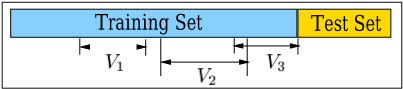
In traditional learning with cross validations, a part of training patterns is reserved a priori in a validation set and not used in learning, and the single objective in learning is to minimize validation errors. Hence, errors measured in validation will not be included in learning. This approach is problematic because it allows only one validation set in learning and excludes patterns in the validation set to be used in learning. As a result, learning may not converge when the time-series contains multiple regimes or when training patterns are scarce.
Based on a constrained formulation, we have proposed a new cross-validation method [Wah and Qian, 2000] that defines multiple validation sets in learning and that includes the error from each validation set as a new constraint (see Figure 1). The use of multiple validation sets is especially suitable for time-series with inadequate training data and for time-series with multiple stationary regimes. The validation error for the a114 ✣ a115 output unit from the ✆ ✣ a115 , ✆ ✜ ✝ ✕ ✼ ✼ ✼ ✕ ✞ , validation set is defined by the normalized mean squared error (✠ ✡ ☞ ✍ ):
✚ where ✗ ✴ ✔ is the variance of the true time series in ✢ ✑ ✔ ✖ ✓ ✕ ✑ ✔ ✖ ✘ ✤ , and ✵ ✔ is the number of patterns in the ✆ ✣ a115 validation set. (Note that errors on the test set in Figure 1 are defined in a similar way.) The constrained formulation then becomes:
where ✒ ✵ (resp. ✒ ✶ ) is the ✠ ✡ ☞ ✍ of the iterative (resp. single-step) validation error, and ♣ , ♣ ✵ ✔ ✖ ✮ and ♣ ✶ ✔ ✖ ✮ are predefined small positive constants.
Eq. (4) is a constrained nonlinear programming problem (NLP) with non-differentiable functions. The formulation, when applied to large time-series predictions, cannot be handled by existing Lagrangian methods that require the differentiability of functions. Methods based on penalty formulations have difficulties in convergence when penalties are not chosen properly. Sampling algorithms [Wah and Wang, 1999] based on our recently developed theory of Lagrange multipliers for discrete constrained optimization [Wah and Wu, 1999], when continuous variables are discretized to floating-point numbers, are too inefficient for solving large learning problems. To address this issue, we present in this paper an efficient learning algorithm called violation-guided back-propagation (VGBP).
2 Theory of Lagrange Multipliers for Discrete Constrained Optimization
To use a Lagrangian method to solve (4), we first transform it into an augmented Lagrangian function:
Since (5) is not differentiable, we discretize variables finely and solve the problem in discrete space using the theory of Lagrange multipliers for discrete constrained optimization [Wah and Wu, 1999]. Algorithm designed to solve constrained NLPs in discrete space can be extended to solve constrained NLPs in continuous space because numerical evaluations of continuous variables using digital computers can be considered as discrete approximations of the original variables up to a computer's precision. The theory in discrete space is summarized in three definitions and one theorem.
Definition 1. ❄ ❅ ❇ ✎ ✸ ✚ is a finite user-defined set of points ✸ ❈ so that ✸ ❈ is reachable from ✸ in one step and that ✸ can reach anypoint in the discreteweight space through ❄ ❅ ❇ ✎ ✸ ✚ .
Definition 2. Point ✸ is a ● ❍ ✡ ❅ ❇ iff (4) is feasible at ✸ and the objective function is the smallest in ① ✸ ④ ▲ ❄ ❅ ❇ ✎ ✸ ✚ . Note that a ● ❍ ✡ ❅ ❇ of (4) is the same as a feasible point.
Definition 3. ☞ ❖ ❅ ❇ ✎ ✸ a80 ✕ ◗ a80 ✚ , a discrete-neighborhood saddle point at ✎ ✸ a80 ✕ ◗ a80 ✚ , satisfies:
for all ✸ ❯ ❄ ❅ ❇ ✎ ✸ ❘ ✚ and all real vector ◗ .
Theorem 1. First-order necessary and sufficient condition on ● ❍ ✡ ❅ ❇ [Wah and Wu, 1999]. A point in the discrete space of (4) is a ● ❍ ✡ ❅ ❇ iff it satisfies (6) for any ◗ ❲ ◗ ❘ , where ◗ ❲ ◗ ❘ means that each element of ◗ is not less than the corresponding element of ◗ ❘ .
The theorem shows that solving (4) in discrete space is equivalent to (the much easier problem of) finding ☞ ❖ ❅ ❇ of (5). Note that the theorem does not hold in continuous space.
3 Violation-Guided Back-Propagation
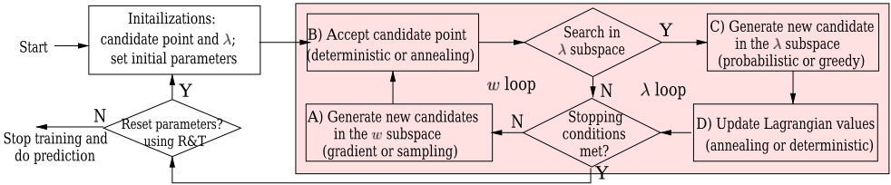
In this section we describe an efficient algorithm to look for ☞ ❖ ❅ ❇ in the Lagrangian space defined in (5). The shaded box in Figure 2 [Wah and Chen, 2000] shows the framework with two parts: one performing descents in the ✸ subspace and another performing ascents in the ◗ subspace. As indicated earlier, random sampling in a Lagrangian space with discrete ✸ is too inefficient. To this end, we propose in Section 3.1 to use BP to compute an approximate gradient direction in order to generate a probe. Since gradient descents may lead to infeasible local minima, we present a new annealing strategy in Section 3.2 to help escape from infeasible points. Last, we exploit special properties in the constrained formulation for ANN learning and present in Section 3.3 a new relax-andtighten (R&T) strategy to successively tighten constraints as more relaxed constraints are satisfied. The R&T strategy is depicted in the two boxes on the left of Figure 2.
3.1 Framework to look for ☛ ☞ ✍ ✎
The ✸ loop in Figure 2 performs descents in the ✸ subspace by generating candidates in Box (A) and by accepting the candidates generated using deterministic or annealing rules in Box (B). Occasionally, the ◗ loop carries out ascents in the ◗ subspace by generating candidates in the ◗ subspace in Box (C) and by accepting them using deterministic or annealing rules in Box (D). In this subsection we present the functions of Boxes (A), (C) and (D) and leave the discussion of Box (B) to the next subsection.
For a learning problem with a large number of weights and/or training patterns, it is essential that the points generated be likely candidates to be accepted. Since (5) is not differentiable, we choose an approximate gradient direction by setting output error ✑ ❈ ✮ ✎ ✑ ✚ ✒ ◗ ✮ ✎ ✑ ✚ ✑ ✮ ✎ ✑ ✚ , applying BP to compute the gradient of the mean squared errors of ✑ ❈ ✮ ✎ ✑ ✚ , generating a trial point using the approximate gradient and step size ✓ , and mapping the trial point to (discretized) floating-point space. In this way, a training pattern with a large error (and its corresponding Lagrange multiplier) will contribute more in the overall gradient direction, leading to an effective suppression of constraint violations,
Step size ✓ used in deriving a candidate point must be dynamic because the same candidate point will be generated repeatedly using a fixed ✓ and a deterministic gradient algorithm. In our algorithm, we generate ✓ uniformly in ✎ ③ ✕ ✓ ✓ ✚ and adapt ✓ ✓ dynamically based on the acceptance ratio ✔ of candidate points generated. The reason for the latter strategy is that a high ✔ indicates that the current direction is promising, leading to increases in ✓ ✓ and larger step sizes. On the other hand, a low ✔ indicates that the step size is too large for the current search terrain, leading to decreases in ✓ ✓ and smaller step sizes. After extensive experiments, we adjust ✓ ✓ as follows:
Box (C) in Figure 2 increases ◗ as follows:
where ♣ is the tolerance defined in (4) and (5). This rule penalizes a violated constraint relative to ♣ . We do not generate ◗ probabilistically because we like their effects on guidance to take place as soon as possible. The deterministic update of ◗ leads to the deterministic acceptance of ◗ in Box (D).
3.2 Probabilistic acceptances in the ✽ subspace
Since the gradient direction computed by BP does not consider constraints due to cross validation and the step size is chosen heuristically, it is possible that a search may get stuck in infeasible local minima. In previous studies, restarts are often used to help escape from such points. However, our experimental results have shown that uncontrolled restarts may lead to loss of valuable local information collected during a search. To solve this problem, we propose an annealing strategy in Box (B) that decides whether to go from current point ✎ ✸ ✕ ◗ ✚ to ✎ ✸ ❈ ✕ ◗ ✚ according to the Metropolis probability:
where ✉ ▲ ✜ ☎ ✆ ✞ ① ③ ✕ ✉ ④ , and ◆ is a parameters introduced to control the acceptance probability.
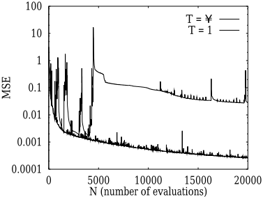
Figure 3 plots the progress of the mean squared errors (MSE) defined in (1) of training an ANN to predict the Mackey-Glass-17 time-series (in short MG17) by using two fixed temperatures: ◆ ✜ ✝ and ◆ ✜ ❖ , respectively. (MG17 is used as a running example throughout this section unless specified otherwise.)
When ◆ ✜ ❖ is combined with restarts, the algorithm accepts every trial point generated in the same way as traditional BP. Figure 3 illustrates this behavior by showing a search that explores a local region in the first 4000 evaluations, got stuck in an infeasible local minimum, and restarted to a new point without keeping any history information.
On the other hand, using ◆ ✜ ✝ allows the search to accept trial points according to (9) and rejects poor points with high probability. Consequently, the algorithm keeps implicitly the history information of points searched in the past and progresses smoothly without escaping into poor regions blindly.
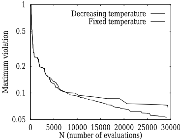
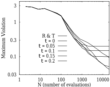
In contrast to conventional annealing schedules that start a search at high temperatures and decrease the temperature to zero as time runs out, we use a fixed temperature throughout the search. A fixed temperature is chosen so that local descents will only be carried out by BP and not by annealing at low temperatures, and that a search will always have an opportunity to explore better regions. Figure 4 shows the improvements in maximum constraint violations when a fixed temperature is used as compared to those at low temperatures using a dynamic temperature schedule.
3.3 Relax-and-tighten (R&T) strategy
It is undesirable to set violation tolerance ♣ ✜ ③ initially in a search because we do not know whether such a violation tolerance can be achieved by the search. Moreover, setting ♣ ✜ ③ will result in considerably large violations in each pattern, leading to large ◗ 's, a rugged search space, and a more difficult search. On the other hand, if we set a loose ♣ ✭ ③ initially, then most constraints can be satisfied easily, and the algorithm can focus on the few patterns with large constraint violations and increase their corresponding ◗ 's.
Another observation is that the progress of a search differs considerably for different fixed ♣ 's. These differences are illustrated in Figure 5 that shows the average maximum violations for different ✵ (number of evaluations) over five independent runs. When ✵ is small, there is little difference in maximum violations. As ✵ is increased, runs with larger ♣ 's have faster decreases in maximum violation than those with smaller ♣ 's. Eventually, all the curves level off when either all constraints are almost satisfied using the specified ♣ or further improvement is impossible using the given ANN topology. The figure also shows a steeper rate of decrease of maximumviolations with larger ♣ 's.
Our proposed R&T strategy exploits the different convergence behavior due to different ♣ 's by dynamically adjusting ♣ during a search in order to achieve the fastest convergence rate through the search. This is done by choosing a loose ♣ initially and by tightening ♣ ✒ ☞ ♣ when the maximum violation of all constraints satisfies ☎ ✈ ✇ ✮ ① ♠ ✮ ✎ ✑ ✚ ④ ♥ ✎ ✝ ✛ ✌ ✚ ♣ , where ③ ✷ ✌ ✷ ☞ ✷ ✝ . In this way, the search will try to use the largest possible ♣ at any time and will switch to a smaller ♣ as the convergence behavior using the original ♣ levels off.
Figure 5 illustrates the behavior of our proposed R&T algorithm. Initially, we set ♣ ✜ ③ ✯ ✎ , leading to the steepest convergence behavior. When the convergence behavior levels off, we switch to ♣ ✜ ③ ✯ ✝ ✸ by tightening the constraints, again leading to the steepest convergence behavior for the range of ✵ used. By repeatedly tightening constraints, the convergence behavior of R&T leads to the envelope of the best convergence behavior at all times.
The choice of the initial ♣ is not critical to convergence as long as it is large enough because the larger the ♣ is, the steeper the curve will be and the shorter the amount of time before it will level off and tighten ♣ . In our implementation, we set initial ♣ ✜ ③ ✯ ✑ ☎ ✈ ✇ ✮ ① ♠ ✮ ✎ ✑ ✚ ④ over all constraints, ☞ ✜ ③ ✯ ✒ ✸ , and ✌ ✜ ③ ✯ ✝ . Around those values, convergence is not sensitive to different ☞ 's and ✌ 's.
The R&T strategy works well on a constrained formulation of ANN learning because all constraints are defined in the same range (limited by the activation function) and all constraints have similar magnitudes. In a general constrained NLP in which constraint violations may vary in large ranges, it will be necessary but difficult to define different amount of relaxations for different constraints. As a result, R&T does not work well in solving general constrained NLPs.
3.4 Parameters in VGBP
In this section, we summarize the values of parameters used in VGBP. First, we set
where ✵ ✔ is the number of training patterns and is known when training begins, ✖ is the range in which ANN outputs are normalized and is set to a default value of one, and ✓ is a constant. ◆ should be proportional to ✵ ✔ because (5) is proportional to ✵ ✔ when all patterns have approximately the same level of violation. Likewise, ◆ should be proportional to ✖ because ✖ affects (5) in a similar manner.
| Method | Number of | Training | Single-step predictions | Iterative predictions | ||
|---|---|---|---|---|---|---|
| weights | 100-1000 | 1001-1050 | 1001-1100 | 1001-1050 | 1001-1100 | |
| FIR network [Wan, 1993] | 1105 | 0.00044 | 0.00061 | 0.023 | 0.0032 | 0.0434 |
| ScaleNet: Multi-scale ANN [Geva, 1998] | N/A | 0.00074 | 0.00437 | 0.0035 | N/A | N/A |
| VGBP (Run 1) | ☎ ✆ ✝ ✞ 461 | ☎ ✆ ✝ ✞ 0.00036 | 0.00043 | 0.0034 | 0.0054 | ☎ ✆ ✝ ✞ 0.0194 |
| VGBP (Run 2) | ☎ ✆ ✝ ✞ 461 | 0.00107 | ☎ ✆ ✝ ✞ 0.00030 | ☎ ✆ ✝ ✞ 0.00276 | ☎ ✆ ✝ ✞ 0.0030 | 0.0294 |
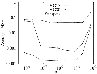
Figure 6 shows the average ✠ ✡ ☞ ✍ 's over 10 runs of VGBP under different ✓ 's for MG17, MG30, and sunspots. Since VGBP is robust over a wide range of ✓ ❯ ✢ ✝ ③ ✤ ✠ ✕ ✝ ③ ✤ ✴ ✤ , we set the default ✓ to be ✝ ③ ✤ ✁ in our implementation.
We further set ✓ ✓ in (7) to be ✝ ✯ ③ . Since ✓ ✓ is adjusted dynamically, its initialization has no significant impact on performance. The setting of ♣ , ☞ and ✌ in R&T has been discussed in Section 3.3.
In short, all the parameters in VGBP are set either by default or automatically, with no tuning required by users.
4 Experimental Results
We have evaluated VGBP with respect to ✠ ✡ ☞ ✍ and the number of weights on several benchmarks.
Laser is a set of chaotic intensity pulsation of an ✵ ☛ ✁ laser in the Santa Fe competition. In that competition, FIRNN [Wan, 1993] took the first place. Table 1 shows that VGBP improves over previous algorithms in terms of prediction quality as well as number of weights used.
Sunspots contains yearly average sunspot numbers from 1700 to 1994. Using data from 1700 to 1920 for training and single-step predictions on four durations, Table 2 shows that VGBP achieves much better performance on all prediction periods, while using less weights than previous designs.
Table 3 compares single-step prediction results using VGBP with previous work on 5 chaotic time series. The two sets of Mackey-Glass and Henon map have one input and one output, whereas Lorenz attractor and Ikeda attractor have one input and two outputs as specified in [Wan, 1997] and [Aussem, 1999].
| Method | a0 | Training | Single-Step Testing | |||
|---|---|---|---|---|---|---|
| 1700-1920 | 1921-55 | 1956-79 | 1980-94 | 1921-94 | ||
| AR(12) | 12 | 0.128 | 0.126 | 0.36 | 0.306 | 0.238 |
| WNet | 113 | 0.082 | 0.086 | 0.35 | 0.313 | 0.219 |
| SSNet | N/A | N/A | 0.077 | N/A | N/A | N/A |
| DRNN | 30 | 0.105 | 0.091 | 0.273 | N/A | N/A |
| COMM | N/A | 0.079 | 0.065 | 0.24 | 0.188 | 0.148 |
| ScaleNet | N/A | 0.086 | 0.057 | 0.13 | N/A | N/A |
| VGBP | ☎ ✆ ✝ ✞ 11 | ☎ ✆ ✝ ✞ 0.0559 | ☎ ✆ ✝ ✞ 0.0337 | ☎ ✆ ✝ ✞ 0.0524 | ☎ ✆ ✝ ✞ 0.0332 | ☎ ✆ ✝ ✞ 0.0397 |
In terms of single-step predictions, Table 3 shows that VGBP uses less weights and achieves impressive ✠ ✡ ☞ ✍ 's one to two orders of magnitude smaller than those of other methods.
Similarly, VGBP achieves much more accurate iterative predictions as compared to those of [Wan, 1997] and [Aussem, 1999]. For example, VGBP was able to achieve iterative-prediction ✠ ✡ ☞ ✍ 's of ③ ✯ ③ ✝ ✑ for MG17 and ③ ✯ ③ ③ ✌ ✎ for MG30, respectively, for the duration 501-600. In contrast, applying Wan's training algorithm on FIR-NN [Wan, 1997] leads to iterative-prediction ✠ ✡ ☞ ✍ 's of ③ ✯ ✑ ✑ ✑ ✎ for MG17 and ③ ✯ ✝ ✎ ✑ ✱ for MG30. Figure 7 plots the iterative predictions of the ANN found by VGBP and that by Wan's algorithm for MG17 and MG30. The figure shows that our iterative predictions are accurate for as many as 100 steps.
In general, it may be hard to predict chaotic time series multiple steps into the future since they are unpredictable by their nature. For this reason, DRNN [Aussem, 1999] did not emphasize prediction performance, especially iterativeprediction performance [Aussem, 2001]. However, our work has shown that it is possible to predict at least the first 100 steps for the Mackey-Glass time series, and better for the other three sets of chaotic time series, although iterative predictions are much harder for the latter. For example, we can achieve an ✠ ✡ ☞ ✍ of only ③ ✯ ✝ ✑ ✌ ✒ for the first 20 steps of Henonmap, whereasWan's algorithmachieves an ✠ ✡ ☞ ✍ of ③ ✯ ✌ ✎ ✸ ✎ .
In short, constrained formulations solved by VGBP lead to superior prediction performance for the benchmarks tested.
@inproceedings{ijcai2001p105,
  title     = {Violation-Guided Learning for Constrained Formulations in Neural-Network Time-Series Predictions},
  author    = {Wah, Benjamin W. and Qian, Minglun},
  booktitle = {Proceedings of the Seventeenth International Joint Conference on
               Artificial Intelligence, {IJCAI-01}},
  publisher = {International Joint Conferences on Artificial Intelligence},
  editor    = {Bernhard Nebel},
  pages     = {771--775},
  year      = {2001},
  url       = {https://ijcai.org/proceedings/2001/105},
}
TY - CPAPER TI - Violation-Guided Learning for Constrained Formulations in Neural-Network Time-Series Predictions AU - Wah, Benjamin W. AU - Qian, Minglun T2 - Proceedings of the Seventeenth International Joint Conference on Artificial Intelligence, IJCAI-01 PB - International Joint Conferences on Artificial Intelligence PY - 2001 SP - 771 EP - 775 UR - https://ijcai.org/proceedings/2001/105 ER -Copied
Machine-readable versions of this paper, for tools and AI agents:





