Temporal Coherence and Prediction Decay in TD Learning

1 Introduction

Two major parameters that control the behaviour of Sutton's [1988] temporal difference algorithm TD(A.) are the learning rate (or step-size), a, and the temporal dis­ count parameter, A..

The choice of these parameters can have a major effect on the efficacy of the learning algorithm, and in practical problems they are often determined somewhat arbitrarily, or else by trying a number of values and 'seeing what works' (e.g. Tesauro [1992]). Another widely used method is to use a learning rate that decreases over time, but such systems still require the selection of a suitable schedule.

Sutton and Singh [ 1994] describe systems for setting both a and A., within the framework of Markov-chain models. However these methods assume relatively small numbers of distinct states, and acylic graphs, and so are not directly applicable to more complex real-world problems . Jacobs [1988] presented the 'delta-bar-delta' algorithm for adjusting a during the learning process. We compared the performance of delta-bar-delta with our algorithm on our sample domain. More recently, Almeida [ 1998] and Schraudolph [ 1998] have presented other methods for a adaptation for stochastic domains and neural networks respectively.

We describe a new system which automatically adjusts a and A.. This system does not require any a priori knowledge about suitable values for learning rate or temporal discount parameters for a given domain. It ad­ justs these parameters according to the learning experi­ ences themselves. We present results that show that this method is effective, and in our sample domain yielded better learning performance than our best attempt to find optimum choices of fixed a and A. , and better learning performance than delta-bar-delta.

2. Temporal difference learning

Temporal difference learning methods are a class of in­ cremental learning procedures for learning predictions in multi-step prediction problems. Whereas earlier predic­ tion learning procedures were driven by the difference between the predicted and actual outcome, TD methods are driven by the difference between temporally succes­ sive predictions.

Sutton's TD(A.) algorithm can be summarised by the following formula. Given a vector of adjustable weights, w, and a series of successive predictions, P, weight ad­ justments are determined at each timestep according to:

where a is the parameter controlling the learning rate, Vw?k is the partial derivative of Pk with respect to w, and P, is the prediction at timestep t. The temporal discount parameter, A, provides an exponentially decaying weight for more distant predictions.

The formula shows that TD(A.) is parameterised by a, the learning rate, and A, the temporal discount factor .

Both parameters, and especially a, can have a major ef­ fect on the speed with which the weights approach an optimum. In Sutton's paper, learning behaviour for dif­ ferent a and A values in sample domains is presented, but no method for determining suitable values a priori is known . Learning rates too high can cause failure to reach stable values and learning rates too low can lead to orders of magnitude more observations being necessary. Methods of choosing suitable a and A values before or during the learning are therefore advantageous. There have been several algorithms proposed for adjusting a in supervised and TD learning: ours is based on a new prin­ ciple that we call temporal coherence.

3. Temporal Coherence: adjusting a

Our system of self-adjusting learning rates is based on the concept that the learning rate should be higher when there is significant learning taking place, and lower when changes to the weights are primarily due to noise. Ran­ dom noise will tend to produce adjustments that cancel out as they accumulate. Adjustments making useful ad­ aptations to the observed predictions will tend to rein­ force as they accumulate. As weight values approach their optimum, prediction errors will become mainly ran­ dom noise .

Motivated by these considerations, our Temporal Co­ herence (TC) method estimates the significance of the weight movements by the relative strength of reinforcing adjustments to total adjustments. The learning rate is set according to the proportion of reinforcing adjustments as a fraction of all adjustments. This method has the desir­ able property that the learning rate reduces as optimum values are approached, tending towards zero. It has the equally desirable property of allowing the learning rate to increase if random adjustments are subsequently fol­ lowed by a consistent trend.

Separate learning rates are maintained for each weight, so that weights that have become close to optimum do not fluctuate unnecessarily, and thereby add to the noise affecting predictions. The use of a separate learning rate for each weight allows for the possibility that different weights might become stable at different times during the learning process. For example, if weight A has become fairly stable after I 00 updates, but weight B is still con­ sistently rising, then it is desirable for the learning rate for weight B to be higher than that for weight A. An additional potential advantage of separate learning rates is that individual weights can be independent when new weights are added to the learning process. If new terms or nodes are added to an existing predictor, independent rates make it possible for the new weights to adjust quickly, whilst existing weights only increase their learning rates in response to perceived need.

The TC learning rates are determined by the history of recommended adjustments to each weight. We use the term 'recommended change' to mean the temporal differ­ ence adjustment prior to multiplication by the learning rate. This detachment of the learning rate enables the TC

algorithm to respond to the underlying adjustment im­ pulses, unaffected by its own recent choice of learning rate. It has the additional advantage that if the learning rate should reach zero, future learning rates are still free to be non-zero, and the learning does not halt.

The recommended change for weight W; at timestep t is defined as :

The actual change made to weight w; after game is:

where a; is the individual learning rate for weight w; and c is a learning rate for the whole process.

For each weight we are interested in two numbers: the accumulated net change (the sum of the individual rec­ ommended changes), and the accumulated absolute change (the sum of the absolute individual recommended changes). The ratio of net change, N, to absolute change, A, allows us to measure whether the adjustments to a given weight are mainly in the same 'direction'. We take reinforcing adjustments as indicating an underlying trend, and cancelling adjustments as indicating noise from the stochastic nature of the domain (or limitations of the domain model that contains the weights) . The individual learning rate, a; for each weight w; is set to be the ratio of net recommended change to absolute recom­ mended change:

with the following definitions and update rules:

r;.1 = recommended change for weight W; at prediction t P1 .. Pend·l are predictions, Pend is the final outcome

The operational order is that changes to w; are made first, using the previous values of N;, A; and a; , then N;, A; and a; are updated. The parameter c has to be chosen, but this does not demand a choice between fast learning and eventual stability, since it can be set high initially, and the a; then provide automatic adjustment during the learning process. All the a; are initialised to I at the start of the learning process.

The foregoing formulae describe updating the weights and learning rates at the end of each sequence. The method may be easily amended to update more fre­ quently (e.g. after each prediction), or less frequently (e.g. after a batch of sequences). For the experiments reported in this paper, update at the end of each game sequence is natural and convenient to implement.

4. Prediction Decay: determining A

We determine a value for the temporal discount pa­ rameter, A, by computing a quantity If/ we call prediction decay. Prediction decay is a function of observed pre­ diction values, indexed by temporal distance between them, described in more detail in appendix A. An expo­ nential curve is fitted to the observed data, and the expo­ nential constant, If/, from the fitted curve is the predic­ tion decay. We set A=l initially, and A= If/thereafter.

The use of A= If/ has the desirable characteristics that (i) a perfect predictor will result in 1f1= 1, and TD(l) is an appropriate value for the limiting case as predictions approach perfection, (ii) as the prediction reliability increases, If/ increases, and it is reasonable to choose higher values of A for TD learning as the prediction reliability improves. We make no claim that setting A=lj/ is optimum. Our experience is that it typically performs better than human-guessed choice of a fixed A a priori. 1

The advantage of using prediction decay is that it en­ ables TD(A.) to be applied effectively to domains without prior domain knowledge, and without prior experiments to determine an effective A. When combined with our method for adjusting learning rates, the resulting algo­ rithm performs better than the comparison method, and better than using fixed rates, in both test domains.

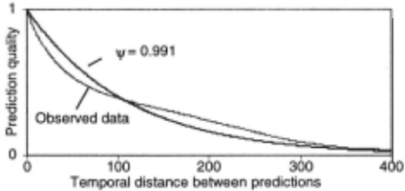
Prediction decay is the average deterioration in pre­ diction quality per timestep. A prediction quality func­ tion measures the correspondence between a prediction and a later prediction (or end-of-sequence outcome). The observed prediction qualities for each temporal distance are averaged. An exponential curve is then fitted to the average prediction qualities against distance (Figure 1 shows an example), and the exponential constant of that fitted curve is the prediction decay, If/. We set the TD discount parameter A , to 1 initially, and A= If/ thereafter. In the experiments reported , If/ (and hence A) were up­ dated at the end of each sequence.

The prediction quality measure, Qd(p, p') we used is defined below. It is constructed as a piece-wise linear function with the following properties:

1. When the two predictions p and p ~ are identical, Qd = 1. (The maximum Qd is I)
2. As the discrepancy between p and p' increases, Qd decreases.
3. When one prediction is I and the other is 0, then Qd = -1 . (The minimum Qd is -1)
4. For any given p, the average value of Qd for all pos­ sible values of p ~ such that 0 ~ p' ~ I, equals 0. (Thus random guessing yields a score of zero.) This property is achieved by the quadratic equations m the definition below.

We achieve all these properties by defining:

1 By expending sufficient computation time to repeatedly re­ run the experiments we found somewhat better values for A..

where:

p is the current prediction, p' is an earlier prediction, and d refers to the temporal distance between p and p'. Predictions lie in the range [0, 1] .

It is assumed that the learning occurs over the course of many multi-step sequences, in which a prediction is made at each step; and that the sequences are independ­ ent. To form a prediction pair, both predictions must lie within the same sequence.

Qd is the average prediction quality over all prediction pairs separated by distance d observed so far. For this purpose, the terminal outcome at the end of the sequence is treated as a prediction. At every prediction, the Qd are incrementally updated.

An example graph from our experimental results is given in Figure 1. This example is typical of the fit to the observed data in the test domain. The exponential curve is fitted to the average prediction quality by minimising the mean squared error between the exponential curve and the observed Qd values. If/ was fairly stable in the range 0.990 - 0.993 during the test runs.

To prevent rarely occurring distances from carrying undue weight in the overall error, the error term for each distance is weighted by the number of observed predic­ tion pairs. Thus we seek a value of 'If which minimises:

where Qd is the average prediction quality for distance d, and Nd is the number of prediction pairs separated by that distance, and 1 is the length of the longest sequence in the observations so far.

In the experiments reported here the value for 1f1 was obtained by simple iterative means, making small incre­ mental changes to its value until a minimum was identi­ fied. Values for IJI(and hence A.) were updated at the end of each sequence.

5. Delta-bar-delta

The delta-bar-delta algorithm (OBO) for adapting learn­ ing rates is described by Jacobs [1988]. Sutton [1992] later introduced Incremental . OBO for linear tasks. The original OBO was directly applied to non-linear tasks, and hence more easily adapted to our test domain. In common with our temporal coherence method, it main­ tains a separate learning rate for each weight. If the cur­ rent derivative of a weight and the exponential average of the weight's previous derivatives possess the same sign, then OBO increases the learning rate for that weight by a constant, 1c. If they possess opposite signs, then the learning rate for that weight is decremented by a proportion, ¢, of its current value. The exponential aver­ age of past derivatives is calculated with (}as the base and time as the exponent. The learning rates are initial­ ised to a suitable value, t<J, and are then set automati­ cally, although the meta-parameters 1\, t/J, (}and tO must be supplied. To adapt OBO to TO domains, we compute a weight adjustment term, and a learning rate adjustment at each timestep, after each prediction, but we only apply the weight and learning rate adjustments at the end of each TO sequence. OBO is very sensitive to its meta­ parameters and prior to our experiments we performed many test runs, exploring a large range of meta­ parameter values and combinations. We used the best we found for the comparison between OBO and TC re­ ported here. Both algorithms update the weights, and the internal meta-parameters, at the end of each sequence.

6. Learning in a complex domain

We tested our methods in a complex game domain. The chosen task was the learning of the values of chess pieces by a minimax search program, in the absence of any chess-related initial knowledge other than the rules of the game.

We attempted to learn suitable values for five adjust­ able weights (Pawn, Knight, Bishop, Rook and Queen), via a series of randomised self-play games. Learning from self-play has the important advantage that no ex­ isting expertise (human or machine) is assumed, and thus the method is transferable to domains where no existing expertise is available. Beat and Smith [1997; 1998] show that, using this method, it is possible to )_earn rela­ tive values of the pieces that perform at least as well as those quoted in elementary chess books. The learning performance of the temporal coherence scheme was compared with the learning performance using fixed learning rates, and with delta-bar-delta.

The TO learning process is driven by the differences between successive predictions of the probability of win­ ning during the course of playing a series of games. In this domain each temporal sequence is a set of predic­ tions for all the positions reached in one game, each game corresponding to one sequence in the learning pro­ cess. The predictions vary from 0 (loss) to I (win), and are determined by a search engine that uses the adjust­ able piece weights to evaluate game positions. The weights are updated after each game.

At the start of the experiments all piece weights were initialised to one, and a series of games were played us­ ing a 5-ply search. To avoid the same games from being repeated, the move lists were randomised. This had the effect of selecting at random from all tactically equal moves, and the added benefit of ensuring a wide range of different types of position were encountered.

6.1 Evaluation predictions

In order to make use of temporal differences, the values of positions were converted from the evaluation provided by the chess program into estimations of the probability of winning. This was done using a standard sigmoid squashing function. Thus the prediction of probability of winning for a given position is determined by:

where vis the 'evaluation value', and f; is the piece count differential for piece type i at the given position.

This sigmoid function has the advantage that it has a simple derivative:

6.2 Results

To visualise the results obtained from the various meth­ ods for determining learning rates, we present graphs produced by plotting weights for each of the five piece values over the course of runs consisting of 2,000 game sequences each. Beal and Smith [ 1997] show that this method is capable of learning relative piece values that compare favourably with the widely quoted elementary values of Pawn = 1, Knight and Bishop= 3, Rook= 5 and Queen = 9. The number of sequences in each run is large enough that the values reach a quasi-stable state of random noise around a learnt value. To confirm that the apparent stability is not an artefact, each experiment was repeated 10 times, using different random number seeds.

Figure 2 shows the average weights achieved using fixed settings of a = 0.05 and A. = 0.95 over a series of 10 runs. These settings offered a good combination of learning rate and stability from the many fixed settings that we tried. A lower learning rate produced more sta­ ble values, but at the cost of further increasing the num­ ber of sequences needed to establish an accurate set of relative values. Raising the learning rate makes the weights increasingly unstable.

Figure 3 shows the average weights produced by the delta-bar-delta algorithm over I 0 runs. For this domain we used meta-parameters of K = 0.035, cp = 0.333, 9 = 0.7 and eo = 0.05, guided by data presented by Jacobs [ 1988] and preliminary experiments in this domain. For A., which DBD does not set, we used A-:0.95 derived from our experience with the fixed rate runs. We tried a number of other meta-parameter settings, none of which performed better than the chosen set. It is possible that a comprehensive search for a better set of meta-parameters might have improved the performance of the delta-bar­ delta algorithm, but given the computational cost of a single run of 2000 sequences, we were unable to attempt a systematic search of all the 'meta-parameter values.

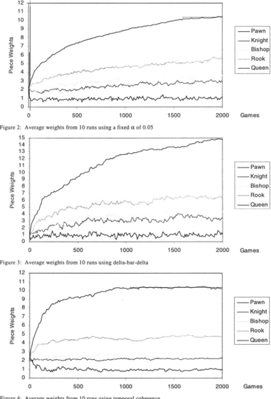
Figure 4 shows the average weights obtained using temporal coherence. It can be seen from the figure that all traces have approached their final values after about 900 sequences (some weights much sooner). Comparing with figures 2 and 3 it can be seen that the TC algorithm is faster to approach final values, and more stable once they are reached. In addition, the traces in figure 4 are smoother than in figures 2 and 3, representing less varia­ tion due to noise in the individual runs.

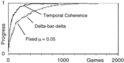
Figure 5 shows the average piece values over 10 runs for the various methods, combined into a single term measuring progress toward the values achieved at the ends of the runs. From this figure we can see that delta­ bar-delta does not improve much on a carefully-chosen fixed learning rate, and that temporal coherence clearly produces faster learning.. The TC and fixed-a final weights were not significantly different.

To confirm that the learning process had produced satisfactory values, a match was played pitting the learnt values against the values widely quoted in elementary chess books Q=9, R=5, N/B=3, P=l. One program used those values, the other used the weights learnt using tem­ poral coherence, as a check that the learnt values were at least as good as the standard ones. In a match of 2,000 games the TC values achieved a score of 58% against the standard values (won=1,119 lost=781 drawn=100).

7. Conclusions

We have described two new extensions, temporal coher­ ence, and prediction decay, to the temporal difference learning method that set and adjust the major control parameters, learning rate and temporal discount, auto­ matically as learning proceeds. The resulting TD algo­ rithm has been tested in depth on a complex domain.

The results demonstrated both faster learning and more stable final values than a previous algorithm and the best of the fixed learning rates. The test domain was one in which values were learnt without supplying any domain­ specific knowledge. We also tested the TC algorithm in a bounded walk domain [Sutton, 1998], and found simi­ lar advantages.

In our comparisons with the delta-bar-delta algorithm, we tried to find good parameter sets for DBD, which requires four meta parameters instead of the one control parameter, a. We tried several different (meta-) pa­ rameter sets in each domain, but were unable to find a set of parameters that improved performance over the results presented in sections 5.1 and 6.2. It is possible that a systematic search for better set of meta-parameters in each of the domains might improve performance. How­ ever, it is a major drawback for the method that it re­ quires its meta-parameters to be tuned to the domain it is operating in. The methods presented here do not require a search for good parameter values.

The experimental results demonstrated that the tempo­ ral coherence plus prediction decay algorithm achieved three benefits: (I) automatic setting and adjustment of parameters (2) faster learning and (3) more stable final values.