Diagrammatic Proofs

1 Introduction

The use of diagrams as reasoning aids has a long his­ tory, but the serious investigation of what is involved in such reasoning is recent. Valuable insights into mixed­ mode or heterogeneous reasoning in which both text and diagrams play essential roles in the instruction of mathe­ matical logic were obtained from the Hyperproof system of Barwise and Etchemendy [Barwise and Etchemendy 95]. Shin [Shin 94] undertook a detailed investigation of how far diagrams and diagrammatic constructions can be used in set theory as an alternative to traditional textual expositions. Sowa [Sowa 84] and the conceptual graph community advocate a diagrammatic approach to knowledge representation and computation. There are also the long-established ER diagrams in databases. For more diverse AI applications, the collection of papers [Glasgow, et. al. 95] is representative of the effort to un­ derstand what constitutes diagrammatic reasoning and Knowledge Systems Group School of MPCE Macquarie University NSW 2109

Australia

the strengths and weaknesses of this mode. Of particu­ lar interest is the idea of "free rides" (see [Shimojima 96] and [Gurr 98] for details), e.g. the processing and un­ derstanding of diagrams that yield facts, relationships, etc. with apparently little effort on the part of humans. Not much of this is well-understood because of the com­ plexity of the tasks and the difficulty of designing ex­ periments to test theories. However, in the specialised domain of mathematical proofs there is the intriguing possibility that the tasks are simpler to understand and experiments may be subject to control protocols. This paper should be read from this perspective. We are for­ tunate that Nelsen [Nelsen 93] has compiled a compre­ hensive collection of such proofs. Indeed, Jamnik, et. al. [Jamnik, et. al. 97] took a number of Nelsen's examples as challenges that required explanation.

We believe that explanation of the efficacy of a dia­ grammatic proof of a mathematical theorem has at least two obligations. The first obligation is to give an account -using standard mathematics, meta-mathematics, logic or computation theory - of why that mode of reasoning is sound. The second obligation is to adduce - or, in the absence of an accepted theory, to conjecture - credible cognitive processes for the "free rides" involved.

The main aim of this paper is to fulfill these obliga­ tions for the chosen examples, and in so doing, pave the way for discovering the principles behind the mechanical generation and/or verification of diagrammatic proofs. Such principles presume an understanding of the afore­ mentioned cognitive processes.

2 Types of Diagrammatic Proofs

Jamnik, et. al., [Jamnik, et. al. 97] have catego­ rized diagrammatic proofs of mathematical theorems ac­ cording to certain characteristics. They identified three categories. In Category 2 which they examined in re­ cent papers (see also [Jamnik, et. al. 98]), the proofs are schematic. While not requiring induction for the particular proof, one is required to generalize on the size of the diagram. Their central result was to show how a constructive w-rule could be invoked to do this. The paradigmatic example is the sum of odd numbers which Nelsen [op. cit.,p.71) attributes to Nichomachus of Gerasa. As we shall be concerned only with Categories

1 and 3 in this paper, we reproduce their descriptions from Jamnik, et. al. [Jamnik, et. al. 97].

Category 1 Proofs that are not schematic: there is no need for induction to prove the general case. Simple geometric manipulations of a diagram prove the in­ dividual case. At the end, generalisation is required to show that this proof will hold for all [parameters]. Example theorem: Pythagoras Theorem.

Category 3 Proofs that are inherently inductive: for each individual concrete case of the diagram they need an inductive step to prove the theorem. Every particular instance of a theorem, when represented as a diagram, requires the use of abstractions to represent infinity. Thus, the constructive w-rule is not applicable here. Example: Geometric Sum.

In this paper we initiate an examination of both these categories.

3 Category 1 Proofs

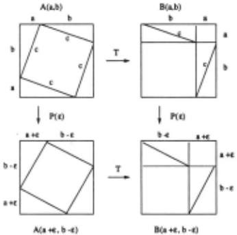
Category 1 proofs somehow require generalization from a specific collection of diagrams. The diagrammatic proof of Pythagoras Theorem, attributed by Nelsen [op. cit.,p.3] to the unknown author of the Chou Pei Suan Ching, is reproduced as the two diagrams A( a, b) and B(a, b) in Figure 1. The dimensions a and b are the lengths of the two sides of the four right-angled congru­ ent triangles with hypotenuse c, a dependent length. In A( a, b), the smaller square embedded in the larger one has side c, so its area is c 2 · It is also the residual re­ gion after the four surrounding triangles are excluded. In B(a, b) we have a transformed version, via diagram­ matic operations T, of A( a, b) in which the triangles have been moved to the positions shown. The residual region outside the triangles, which must have the same area as the one before, are now the two small squares with areas a 2 and b 2 · This proves the theorem for the specific case of these linear dimensions a, b and c.

We propose two solutions to the problem of general­ ization using this example as a paradigm. The first relies on a notion of continuity, while the second is the analog of a powerful meta-theorem in logic. Both of these have precursors in the recent discussion by Hayes and Laforte lHayes and Laforte 98].

The continuity argument has two parts. The first is illustrated in Figure 1 via two additional diagrams A( a+ t:, b-t:) and B(a+t:, b-t:). What is argued here is that the second two diagrams are perturbed versions, via a map P(t:), of the first two, but the same transformation T relation holds. In fact, this can be made precise by saying that the diagrams commute as indicated. This argument shows that the relative ratio a:b is not material, but does not meet the criticism that an absolute magnitude for, say a, is used in the diagram. To meet this we need the second part, which is a scaling argument. That is, to the A( a, b) and B(a, b) diagrams and the operations T , we have a scaled counterpart A(ra, rb) and B(ra, rb) with the same operations.

The second solution, analogous to logic, is the dia­ grammatic version of the theorem called "generalization on constants", also known as the Theorem on Constants (TOC for short). One statement of it (see, e.g. [Shoen­ field 67]) is as follows. Suppose r is a set of formulas and a(x) is a formula with free variable x, and the con­ stant d does not appear in any formula in r. Further' suppose r 1- a[x/d], where the notation a[x/d] signifies the substitution of d for x in a(x). Then we may infer r 1- a(x), and hence r 1- 'v'xa(x).

The discussion below is an outline of how the TOC is applied. The details require attention to the admissible operations on, and inferences from, diagrams; these we postpone to a later paper, but see [Hayes and Laforte 98] for some current insights.

The relevance of the TOC as a response to specificity of the diagrammatic proof of the Pythagoras Theorem lies in the implicit hypotheses r of the proof. We enu­ merate some members of this r: first, there are the Euclidean geometric propositions used, e.g., properties of triangle congruence, the sum of angles of any trian­ gle being 180 degrees, properties of squares, invariance of shapes and areas under rotations and translations. There are also some algebraic identities involving addi­ tions and subtraction of areas, and formulas about the area of any square given the length of its side. None of these mention the constants a, b and c. The con­ struction of diagram A( a, b), and the subsequent opera­ tions (call them T) to transform it to diagram B(a, b), are the steps in the diagrammatic proof. The conclu­ sion of the proof is a 2 + b 2 = c 2 , in symbolic notation r C> a 2 + b 2 = c2, where none of a, b or c occur in r. Here C> is the diagrammatic analog of textual proof (i.e., 1-) in diagrams, principally diagrammatic operations sup­ plemented by reasoning about invariants like areas, etc., the details of which we will elucidate in a future paper. The TOC now authorizes generalization of the conclu­ sion a 2 + b 2 = c 2 to arbitrary values for these constants.

These two responses to Category 1 diagram specificity extend to many other proofs in which ostensibly par­ ticular dimensions are named, e.g., Nelsen's own dia­ grammatic proof [op. cit.,p.22) of Diophantus' "Sum of Squares Identity".

4 Category 3 Proofs

The main feature of Category 3 proofs is an ellipsis, the classical "· · ·" notation used in suggesting the infinite completion of, say, a series such as a0 + a1 + a2 · · ·. This ellipsis is used in Category 3 diagrams to similarly sug­ gest that the reasoning applied so far to a finite diagram can be successfully completed to infinity by some implicit induction. The most well-known example of this is the diagrammatic proof of the sum of the geometric series 1/2, 1/2 2 , 1/2 3 , · · ·, attributed by Nelsen [op. cit.,p.118) to Page. It is reproduced here as diagram A in Figure 2.

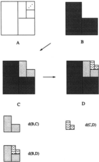
We will now provide justifications for the diagram­ matic steps in the proof, and a semantics for the ellipsis in the diagram. The key idea is to view the completed square as the limit of a sequence of constructions, each of which is a "monotonic" and "Markovian" addition to its predecessor. It is monotonic because each construction stage adds new information that is distinctly represented without retracting old information. It is Markovian be­ cause only the most recent piece of information (con­ struction) is used to construct the next one. The usual diagram with its ellipsis notation is reproduced as dia­ gram A in the figure. The diagram B corresponds to the sum 81 = 1/2 + 1/2 2 . The next diagram C corresponds to the sum (1/2 + 1/2 2 ) + (1/2 3 + 1/2 4 ) = 81 + 82 where 82 abbreviates the second grouping of summands. Each group is colored differently for ease of viewing. Pro­ ceeding likewise, the diagram D corresponds to the sum 81 + 82 + 83 where 83 = (1/2 5 + 1/2 6 ).

4.1 Meaning of the Ellipsis

This subsection assumes some mathematical background that can be found in standard texts such as [Simmons 84). Let us denote by Ai the area corresponding to the summand 8i, i.e., each Ai is an L-shaped region typi­ cally indicated by the differently colored pieces in Fig­ ure 2. The regions can be placed in the first quadrant of co-ordinate axes so that the initial A1 diagram (B in Figure 2) has the origin at its left bottom corner, and the X- andY-edges have length 1. The second region A2 will have its left bottom corner at the point (1/2, 1/2) , and edge lengths 1/2. With this convention, each L­ piece in the later pictures can be described as an affine transformation of the preceding L-piece.

Identifying the L-piece A~e with the co-ordinates of its points, this transformation T can be specified as follows, where d~e is the (co-ordinates of the point at the) left bottom corner of A~e:

The diagram D in Figure 2 can then be denoted as a union A1 U A2 U A3 , which by the definition of the affine transformation can equivalently be written as (I U T U T 2 )A1 , where I is the identity operator. Using this notation as a basis we can express the progression from one diagram to the next as a larger transformation F as follows:

This is the formal expression of the geometric intuition that the next diagram in the sequence is obtained by gluing a smaller (scaled and translated) L-shape onto it at the appropriate corner, making explicit its Markovian character.

There is an obvious way to describe the difference be­ tween, say, diagrams B and C, which is just the addi­ tional L-piece A2 added to B to yield C. This way to view the difference between two diagrams by observing the difference in regions they occupy is a special case of the measure J.L of the symmetric difference between two sets d(X, Y) = J.L((X U Y) \(X n Y)). It is well-known that this is a metric. Thus, the collection of diagrams is a metric space under the d metric. It is therefore possible to consider sequences of such diagrams and ask if such sequences converge under this metric. We have observed in examples of proofs involving ellipses, the collection of diagrams has been broad enough to guarantee that con­ vergent sequences have a limit that is also a diagram in the collection. Formally this says that the diagram space is a complete metric space.

A map G : U -+ U on a metric space U with metric d is a contraction if for all X, Y d(GX, GY) ~ k · d(X, Y) for some k < 1. The Banach Fixed Point (BFP) theorem says that a contraction G in a complete metric space has a unique fixed point, i.e. there is one, and only one, X0 such that G(X0 ) = Xo. Moreover, this fixed point can be constructively obtained from an arbitrary initial point Y by repeated application of G starting from Y, i.e., X0 = limn-+oo Gn(Y). This theorem cannot be directly applied to explicate the efficacy of the diagrammatic proof, but a weaker form of it is relevant. The weaker statement (WFP) still relies on G being a contraction on a sub­ space Yt , Y2 · · · , consisting of the terms in the sequence generated by G starting from a given initial point Yo. Such a sequence will still converge to a fixed point, a re­ sult that follows directly from the standard proof of the BFP theorem.

Observation 1 The transformation F defined above on the space ofT -generated L-shapes is a contraction map. Hence it has a unique fixed point, which is the square A in Figure 2.

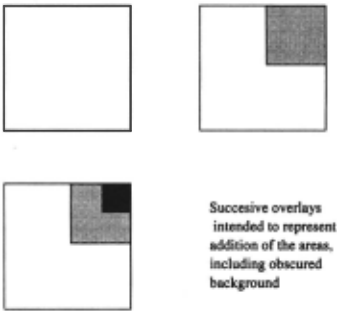
The fact that the general form of the BFP is not helpful in explicating the visual persuasiveness of this diagrammatic proof suggests some cognitive hypotheses that cry out for testing. To .explain the hypotheses, let us examine the transformation F more closely. Suppose the initial diagram is not a unit edge L-shape but a unit square instead. The underlying transformation T as de­ fined before will now work on this square to produce a scaled version of it, then translate this version so that its top right corner coincides with that of the original square. Figure 3 shows the first three members of this sequence. Now, if this is intended to represent the sum of the geometric series 1 + 1/2 2 + 1/2 4 · · ·, we have tore­ define the transformation F to be not the union of the diagram sequence as before, but the sum of the overlaid areas, so that multiple overlays are counted area-wise as many times as they occur. With this re-definition the WFP theorem will still hold, so convergence is guar­ anteed. But unlike Figure 2, the corresponding visual task is no longer easy. Indeed, the area addition at each stage in Figure 3 is not monotonically distinct in terms of representation, as each new piece intersects prior pe­ ices. The crucial difference from Figure 2 appears to be this - the set unions for the L-shaped sequences in Fig­ ure 2 are disjoint unions, that moreover are contiguous, so that sums of areas are easy to see. We therefore con­ jecture that disjoint unions, especially contiguous ones, are free ride features.

There is an important point we note about the choice of the initial shape fed into the constructor T. In Figure 2 we chose an L-shape. We could have conceivably cho­ sen, say, the left tall rectangle in diagram B. If we did that, then the second stage will be the addition of the right square in diagram B. This leads to a more com­ plex constructor T which has to be decomposed into two stages - it is no longer Markovian in the strict sense, but is nevertheless still finite memory. In essence, the choice boils down to how long a preceding sequece is needed to define the next piece( s) of the sequence.

So that we can use "· · ·" as a meta-notation in our description of ellipses, it is convenient to adopt the al­ ternative notation &c to denote the ending ellipses sig­ nifying continuation to the limit in both diagrams and sequential expressions. With these remarks, we propose that the the semantics of ellipses be as follows.

Definition 1 We interpret the meaning of the ellipsis &c in the diagram A1 U A2 &c to be a constructor func­ tion application written in "suffix form" with argument the diagram At U A2, and whose value is the diagram At UA2 UA3 &c. More generally, &c denotes a function &c defined as follows: the diagram A1 U · · · U AA: &c has the intended meaning &c (At U · · · U AA:) which evaluates to the diagram F(At U · · · U AA:) &c.

This has the effect of making &c denote a "lazy ex­ pander" of the finite diagram so far constructed. A more formal approach to the semantics of &c appeals to the notion of recursive domains [Stoy 77] in which the dia­ grams are the solutions (up to isomorphism) of the do­ main equation

and the "completed" (infinite) diagram, i.e., the square in this case, is the least upper bound of these solutions. Here the function end extracts the last component of the instance of Aexp, and l±l is the ordered union operation.

4.2 Construction Invariants

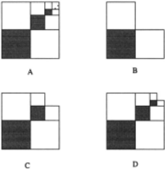
Another example of a Category 3 proof, attributed by Nelsen (op. cit.,p.121] to Ajose, is shown in Fig­ ure 4. The diagram A in it is the proof of the sum 1/2 2 + 1/2 4 + 1/2 6 &c = 1/3. Diagrams B, C and D show the analogs of the construction leading to diagram A as was explained for the proof in Figure 2, with the L-shapes as before. As the semantics for the ellipsis &c is similar to that above, we will omit it. However, in this proof a new feature is present that requires justification. As can be seen from the diagrams B,C and D, we have at each stage to "see" that the colored area is 1/3 of the total area (L-shapes) constructed so far, and that eventually the total area is 1. That the eventual area is 1 is reached exactly as in the proof in Figure 2. How do we account for the other piece of inference - that the colored area is always 1/3 of the total? We propose that the underlying idea is a construction invariant. This is closely related to the idea of a loop invariant in the se­ mantics of programming languages. There, a first-order formula ¢ is a loop invariant in loop L if its truth at the point of entry into the loop guarantees its truth at the end of it, denoted <P :J [L]¢. Likewise, in the present construction, let ¢[area] stand for the statement: "col­ ored area = 1/3 total area". Then we have the visual proof rule: { ¢[A1 U .. · U Ak] :J ¢[F(A1 U .. · U Ak)]} :::> ¢[A1 U · · · U Ak &c], where F is the one-step constructor above.

The visual proof rule is a formal statement of the con­ jecture that such uniform invariants across uniform con­ structions are inductive "free rides". In other words, such proof rules capture the essence of cognitive induc­ tion in diagram completions or fixed points.

5 Schroder-Bernstein Theorem

As yet another instance of a Category 3 type proof which illustrates the ellipsis and construction invariant features, we will now examine the diagrammatic aid to the eroof of the Schroder-Bernstein theorem in set the­ ory [Kamke 50]. This theorem states that if there is an injection 'ljJ from set S into set U and also an injection x from set U into set S, then the sets have the same car­ dinality, i.e., there is a bijection 11 between them. The usual proof uses a "back-and-forth" argument, but there is a less well-known proof that establishes a (apparently stronger, but actually equivalent) statement which im­ plies the theorem, and is arguably easier to expound. This statement is as follows: If there is an injection 1r from set S into a proper subset A1 of itself, then there is a bijection between S and all subsets S1 such that A1 c S1 c S. It is this latter statement whose proof is usually accompanied by a diagram, the appeal to which is inessential only to the most experienced and sophisticated of set theorists. All others (the authors included) appear to find the diagram indispensable. The use of this diagram further exhibits some of the properties discussed in the preceding sections, and invites similar conjectures.

..-----------'

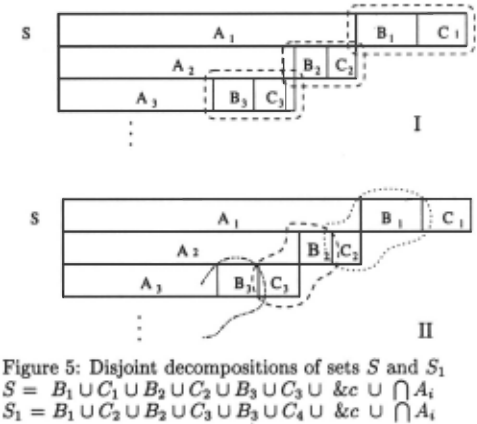
Figure 5 illustrates the reasoning steps. It is adapted from [Kamke 50]. The successive arguments are repre­ sented by different views of the same set, each view being a strip partitioned as shown. For instance, the original setS is (represented by) the first strip, with the labelled partitions A1, B1 and C1 having the following roles: A1 is as above, being the assumed injective image subset of S, i.e. A1 = 1r(S); A1 u B1 = S1; and C1 is what is "left over". Now, the next strip has partitions A2, B2 and C2 with the following roles: A2 = 1r(AI), B2 = 1r(B1), and C2 = 1r( C1). The subsequent layers are interpreted likewise.

The diagram I shows a way to decompose the set S . It yields the equation S = B1 U C1 U B2 U C2 U B3 U C3 &c UnA,. The diagram II shows a way to decom­ pose the set S1 (= A1 U B1). It yields the equation S1 = Bt U C2 U B2 U C3 U B3 U C4 &c U n A, . Then by aligning these equations as indicated in Figure 5, we see that the disjoint components are in one-to-one cor­ respondence with each other (bearing in mind that by assumption Ck+l = 1r(Ck)), thereby establishing the bi­ jection between S and S1 as required.

What devices have been used in this appeal to the diagrams? First, the layout of the successive strips em­ phasized the disjoint components, much as in the proofs of the sums of series above. Second, the decompositions used the elliptical &c as above. Third, the apparently textual alignment of the two decompositions were used to argue for extension of pairwise correspondences be­ tween components to the entire set union. We submit that the third device is at least as much diagrammatic as it is textual, depending as it were on appeal to a linear layout and the elliptical &c for its "free ride" cogency.

We note in particular the implicit appeal to an in­ variant and a visual proof rule. Let 4>[81, 82] stand for the statement: 81 ~ 82, where ~ means a termwise 1-1 correspondence between the two sequences 81 and 82 · Then we have the visual proof rule: { 4>[8t, 82] :::> 4>[F([81), F(82)]} :::> 4>[81 &c, 82 &c], where F is the one­ step constructor for extending the partitions to the next layer.

6 Conjectures for "free rides"

In the preceding analyses we suggested a number of fea­ tures of diagrams in mathematical proofs that seem to resonate with cognitive ease of processing. It is conve­ nient to summarize them here as challenges for controlled experiments. If validated, they can form the basis for the automation and generation of diagrammatic proof systems, and of related HCI designs for diagrammatic reasoning. Invalidation of any of them will prompt al­ ternatives, and certainly prevent some blind alleys from being pursued. Some diagrammatic features that facili­ tate proofs are conjectured to be:

• Continuous transformations of proof constructions.
• Disjoint unions or decompositions.
• Contiguous pieces in these unions.
• Monotone sequences of areas with a "Markovian" uniform rule that generates the next element from the last one.
• Limits are upper or lower bounds of such sequences.
• Simply shaped upper or lower bounds.
• Contractive mappings with simple (see below) met­ rics like symmetric difference.
• Ellipses represent implicit uniform constructions with lazy evaluation semantics.
• Simply perceived relations between areas.
• Relations true in the limit are exactly those invari­ ant with respect to one step uniform (Markovian) constructions.

We end this concluding section by remarking on met­ rics for sets. It would not have escaped the attention of readers familiar with work in fractals [Peitgen, et. al. 92] that diagrams such as Figures 2 and 4 are reminiscent of such recursively generated images. In fractal topology, the convergence metric normally used is the Hausdorff metric. We · believe that this is not a "free ride" metric, and hence is not simple, for reasons that we will explain elsewhere.

7 Acknowledgements

We thank Donald Michie, Pavlos Peppas, Yusuf Pisan and Yan Zhang for their comments on earlier versions of this paper. This research is supported in part by a grant from the Australian Research Council.