
Utilizing Device Behavior in Structure-Based Diagnosis
Proceedings of the Sixteenth International Joint Conference on Artificial Intelligence. Qualitative Reasoning and Diagnosis. Pages 1096-1100.
© 1999 International Joint Conferences on Artificial Intelligence
Abstract
Structure-based approaches to diagnosis provide useful computational guarantees based on a device structure. In particular, these approaches can identify device structures for which the complexity of model-based diagnosis is guaranteed to be linear. Structure-based approaches, however, can fail to answer even the simplest diagnostic queries if the device structure is not well behaved (strongly connected) . We show in this pap er that this deficiency can be addressed to a reasonable extent by utilizing device behavioral properties (its component models in particular) which are typically ignored by structure-based approaches. Specifically, we prese nt a structure-based algorithm for diagnosis which takes advantage of a device behavior and then present experimental results indicating th at our algorithm can lead to significant (orders-of-magnitude) savings over pure structural approaches when applied to strongly connected dev ic es.
- Darwiche, 1998) Adnan Darwiche. Model-based diag- nosis using structured system descriptions. Journal of Artificial Intelligence Research, 8:165-222, 1998.
- Darwiche, 1999) Adnan Darwiche. Compiling knowl- edge into decomposable negation normal form . Tech- nical Report R-262, Cognitive Systems Laboratory, UCLA, 1999. IJCAI
- Dechter and Dechter, 1996) Rina Dechter and Avi Dechter. Structure-driven algorithms for truth main- tenance. Artificial Intelligence, 82:1-20, 1996.
- Geffner and Pearl, 1987) Hector Geffner and Judea Pearl. An improved constraint-propagation algorithm for diagnosis. In Proceedings of IJCAI, pages 1105- 1111, Milan, Italy, 1987.
- Hamscher et al., 1992) Walter Hamscher, Luca Con- sole, and Johan de Kleer. Readings in Model-Based Diagnosis. Morgan Kaufmann Publishers, Inc., San Mateo, California, 1992.
- Jensen et al., 1990) F. V. Jensen, S.L. Lauritzen, and K.G. Olesen. Bayesian updating in recursive graphical models by local computation. Computational Statis- tics Quarterly, 4:269-282, 1990.
- Pearl, 1988) Judea Pearl. Probabilistic Reasoning in Intelligent Systems: Networks of Plausible Inference.
References were extracted automatically from the PDF and may contain errors.
Full text extracted automatically from the PDF; figures, tables and equations may differ. The PDF is the version of record.
1 Introduction
The utilization of problem structure in automated rea soning has become a major computational technique in certain communities and is gaining momentum in oth ers. In probabilistic reasoning and constraint satisfac tion, structure is the main aspect of a problem which is used to control the complexity of inference [Dechter and Dechter, 1996; Jensen et al., 1990; Pearl, 1988]. In probabilistic reasoning, structure refers to the topology of a Bayesian network, and in constraint satisfaction it refers to the topology of a constraint network. Structure based reasoning has also been introduced to model based diagnosis, where structure refers to the intercon nectivity of device components [Hamscher et al., 1992; Dechter and Dechter, 1996; Geffner and Pearl, 1987; Darwiche, 1998] .
One of the most interesting aspects of structure-based diagnosis is that it ties the complexity of computing di agnoses to a very intuitive measure: component inter connectivity. As it turns out, the less connected a device is, the easier it is to diagnose using structure-based methods. The connectivity of a device structure is typ ically summarized by a measure known as the structure width. It is well known that the best-case and worst-case complexities of standard structure-based algorithms are exponential (only) in the width of a device structure. Therefore, if the width is small, all is well. However, if the device structure has a large width, then structure based algorithms are effectively non-usable.
This is probably one of the greatest challenges to structure-based reasoning especially that some problems which are known to be easy (such as inference with Horn clauses) can sometimes be posed as problems with com plex structures; therefore, making them intractable to structure-based methods. Stated differently, one can identify problems that have a varying level of difficulty, yet posses the same structure. This means that the diffi culty of a problem cannot be measured only by its struc ture. It also means that some non-structural properties must be appealed to if one is to optimize the performance of structure-based methods.
The contribution of this paper is in pursuing this in tuition in the context of model-based diagnosis. Specifi cally, we provide a structure-based algorithm for model based diagnosis which exploits non-structural properties of a device. The properties we exploit are the behav ioral models of device components, which are typically ignored by structure-based methods.
Our refined algorithm still maintains the standard worst-case complexity of structure-based methods, but its average-case complexity appears to be significantly better as illustrated by our preliminary experimental results. According to these results, our . refined al gorithm can lead to orders-of-magnitude savings over pure structure-based methods especially when the de vice structure is strongly connected.
This paper is structured as follows. Section 2 presents some technical preliminaries which are needed to phrase the model-based diagnosis problem formally. Section 3 discusses standard approaches to structure-based diag nosis, explaining their use of a device structure and stressing their non-use of a device behavior. Section 4 turns to the basic intuition underlying our use of a device behavior where we introduce decomposition trees, which are a key tool we shall use in realizing our intuitions. Section 5 presents the technical details of our approach and discusses our experimental results. Section 6 closes with some concluding remarks.

2 Model-Based Diagnosis
Our goal in this section is to present a particular for malization of the model-based diagnosis problem. Our formalization is not very standard, but it appears cru cial to exposing the intuitions behind structure-based approaches and our proposed extension to them.
Components: We start by defining a device compo nent cas an object which is characterized by an id, a set of ports, and a diagnosis function. Specifically, id(c) is a number representing a unique identifier for the com ponent; ports(c) is a set of variables (with finite values) representing the component's inputs and outputs; and Dg(c, a) is a function capturing the health of compo nent c given an instantiation a of its ports. 1 The value of Dg ( c, a) is { { id (c)}} if instantiation a is inconsistent with the normal behavior of component c and is { {}} otherwise.
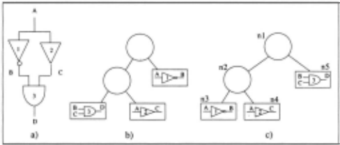
Consider the device in Figure 1 for an example. Let c refer to the first buffer. Then id(c) = 1, ports(c) = {A, B} and Dg(c, a) = { {1}} if a instantiates A and B to different values and Dg(c, a) = { {}} otherwise.
Devices: A device is defined as a set of components c1, ... , Cn. For example, the device in Figure 1 is defined by the set c1, c2, c3, c4, which refer to the four buffers from left to right, respectively. Here, ports(cl) = {A,B} and ports(c2) = {B,C}. Note that one can figure out how components are interconnected by examining the components' ports.
Model-Based Diagnosis: A key question of concern to model-based diagnosis is this: Given a device d = c1 , ... , Cn and an instantiation f3 of some of the device ports, compute the diagnoses consistent with d and /3.
Our goal in the remainder of this section will be to present a simple, brute-force method for answering this question. We shall then argue that structure-based methods refine this method by exploiting device struc ture. Our proposal will then be presented as a further refinement of this method based on device behavior.
Our treatment will make two assumptions: (1) com ponents have no fault modes (they are either broken or ok); and (2) only minimum-cardinality diagnoses are of interest. The first assumption simplifies the discussion considerably but without reducing the generality of our treatment. The second assumption, however, (or a simi lar assumption for preferring some diagnosis over others) is crucial to the techniques we shall propose.
1 An instantiation of a set of variables is an assignment of values to these variables.
The brute-force method for computing minimum cardinality diagnoses is based on diagnosis-sets:
- A diagnosis is a set of component IDs. Example: {1, 3} is a diagnosis with respect to the device in Figure 1. It indicates that components 1 and 3 are faulty.
- A diagnosis-set is a set of diagnoses with equal car dinalities. The cardinality of a diagnosis-set is the cardinality of any of the diagnoses it contains. Ex ample: { {1, 4 }, {2, 4}, {3, 4}} is a diagnosis-set with cardinality 2. It indicates three possible problems, each involving two faults. 2
- The union of two diagnosis-sets is defined as follows:
- The Cartesian Product of two diagnosis-sets is:
Note that the diagnosis function Dg(c, a), which we in troduced earlier, returns a diagnosis-set representing the health of component c given an instantiation a of the component ports.
Computing minimum-cardinality diagnoses can be viewed as extending the diagnosis function Dg to sets of components (devices) . We shall see that this is straight forward given the above operations on diagnosis-sets.
We will first extend Dg while assuming that a is an instantiation of all of the device ports. Specifically, let d = { c1, ... , Cn} be a device and let a be an instantiation of all of d's ports. It should be easy to verify that
represents the minimum-cardinality diagnosis for device d and instantiation a. Consider Figure 1 and let a be the instantiation A0B1 C0D1E1. We have three faults here involving Buffers 1, 2 and 3:
2 Diagnosis-set {} has cardinality oo by definition.
3 Note that Card(s 1 n s2 ) = Card(s!) + Card(s2).
Suppose now that a: is an instantiation of only a subset of the device ports ports (d). It is not hard to verify that
is the set of minimum-cardinality diagnoses for device d and instantiation a:. Here, /3: ports(d) I a: means that /3 is an instantiation of ports(d) which is consistent with Q:.
Given the notions above, the key question of concern to us here is: Given a device d = {c1 , ... ,cn} and an instantiation a: of some of its ports, compute Dg(d, a:) as defined by Equation 2 as efficiently as possible. In the following section, we show the key technique used by structure-based approaches to perform this compu tation. We then follow by our own proposed techniques for improving on this computation.
3 Structure-Based Diagnosis
Structure-based diagnosis systems can be viewed as eval uators of Equation 2 based on the following theorem:
Theorem 1 Let dx and dy be two disjoint sets of com ponents and let d = dx U dy. Then
Intuitively, the theorem shows how one can decompose a diagnostic query with respect to a device d = dx U dy into a set of simpler diagnostic queries with respect to the smaller devices dx and dy. Moreover, this decom position is exponential only in the number of common ports between sub-devices dx and dy.
We have a number of observations about this theorem. First, if applied recursively, it can reduce the computa tion of any diagnosis-set of the form Dg(d, .), where d is a device, into the union and product of diagnosis-sets of the form Dg ( { c}, . ) , where c is a component. Second, the amount of work to compute Dg(d, .) by Theorem 1 can be measured by the number of union operations per formed during the application of the theorem. Third, if it is possible to decompose the components of a device into sets which share a small number of ports, then di agnosing such a device is easy according to Theorem 1.
The main technique underlying structure-based meth ods is to compute good device decompositions and use them to apply Theorem 1 or a variant. Moreover, the main technique used for obtaining such decompositions is to compute a join tree for the device structure [Dechter and Dechter, 1996; Darwiche, 1998].
We will not discuss jointrees in this paper since we will not be using them in our approach. Instead, we will use a simpler variant on jointrees, called decomposition trees, which we introduce later.
We are now ready to introduce the key observation underlying our contribution in this paper. There are two ways to reduce the number of union operations performed while applying Theorem 1; one is structural, the other is behavioral:
- Structural: Minimize the common ports between de vices dx and dy;
- Behavioral: Skip any instantiation /3 for which Card(Dg(d, fJo:)) > Card(Dg(d, a:)) because the contribution of Dg(d,jJa) in this case will be ig nored by the union operation.
The first method is structural because it can be achieved by reasoning about the structure of the device. The second method is behavioral because it requires knowl edge of the specific components comprising the device and cannot be accomplished based on the device struc ture alone. In particular, whether Card(Dg(d, fJo:)) > Card(Dg(d, a:)) holds depends on the diagnosis function Dg(c, .) associated with each device component c. This behavioral dimension for optimizing the application of Theorem 1 can be formalized by the following refined version of the theorem:
Theorem 2 Let dx and dy be two disjoint sets of com ponents and let d = dx U dy . Then
This is exactly like Theorem 1 except that we have added an extra condition on the instantiation /3.
Whereas structure-based methods have been mainly concerned with reducing the size of ports(dx) nports(dy) - therefore, reducing the number of instantiations f3 to consider - by appealing to structural device properties, our focus will be on identifying those in stantiations /3 that do not satisfy the extra condition Card(Dg(d,jJa)) = Card(Dg(d,a)). For this we must consult non-structural properties of devices. This new technique, as we shall demonstrate, can lead to signifi cant savings.
The next section introduces decomposition trees which allow us to provide a simple implementation of Theo rem 1. We then follow by refining the algorithm to reflect the improvement introduced by Theorem 2.
4 Decomposition Trees
A decomposition tree for a device is a full binary tree whose leaves correspond to the device components; see Figure 2. A decomposition tree is simply a control strat egy for applying Theorem 1. To be employed for this purpose, however, we must associate a few properties with each node N in the tree. First, for a leaf node N, comps(N) d~ {c}, where cis the component asso ciated with node N. Second, for an internal node N, N1 and Nr . are the left and right children of N, respectively, and comps(N) d~ comps(Nl) U comps(Nr)· Fi nally, for any node N, ports(N) are the ports of com ponents appearing in comps(N). For example, in Fig
ure 2(c), ports(n3 ) ={A, B} and ports(n2) ={A, B , C}.
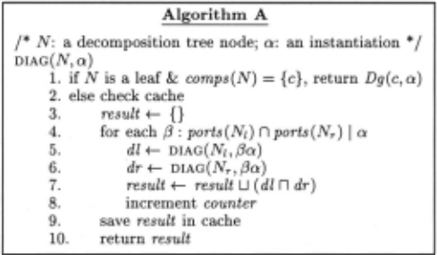
Here is the intuition behind a decomposition tree. The root node N represents the whole device which is decom posed into two sub-devices, one represented by Nl and another by Nr. Therefore, to compute minimum cardi nality diagnoses, all we have to do is apply Theorem 1 with dx and dy being comps(Nl) and comps(Nr)· Fig ure 3 presents a simple recursive algorithm (based on Theorem 1) for computing minimum-cardinality diag noses given a device decomposition tree.
We have a number of observations on Figure 3. First, note the boundary case where node N is a leaf node. In such a case, component c is associated with node N and we simply return Dg(c, a), which is either { { id(c)}} or { {}} as stated earlier. 4 Second, we have included a counter on Line 8 to count the number of union op erations performed. This is needed to explain our ex perimental results later. Finally, we have included a caching mechanism on Lines 2 and 9 because, by defi nition, two calls DIAG(N, a) and DIAG(N, a') will return equal diagnosis-sets whenever a and a' agree on the val ues of ports(N). Therefore, we keep a cache at each node N which stores the result of call DIAG(N, a) indexed by the projection of instantiation a on ports(N). If another call DIAG(N, a') is made, the cache is checked first to see whether we have an entry for the projection of a' on ports(N). If there is, the entry is returned. Otherwise, the call DIAG(N, a') recurses.
4 When a call DIAG(N, a) is made on the root node, we assume that a is an instantiation of all input and output ports of the device. This guarantees that when we reach the boundary case on Line 1, a would instantiate all ports of the component c.
The quality of a decomposition tree is measured by its width and the complexity of Algorithm A is linear in the number of nodes in the decomposition tree and exponential only in its width. Following is the formal definition of a decomposition tree width.
Definition 1 Let N be a node in a decomposition tree T . The cluster of node N is defined as follows . If N is a leaf node, then its cluster is ports ( N). If N is an internal node, then its cluster is the set of ports that appear either above and below node N in the tree, or in the left and right subtrees of node N. The width of a decomposition tree is the size of its maximal cluster minus one.
Consider node n2 in Figure 2(c). Then {B, C, D} and {A, B, C} are the ports that appear above and below node n2 , respectively; Moreover, {A, B} and {A, C} are the ports that appear to the left and right of n2, respectively. Therefore, the cluster of node n2 is ({B,C,D}n{A,B,C})u({A,B}n{A,C}) = {A, B,C}.
Theorem 3 LetT be the decomposition tree used in Al gorithm A. The running time of Algorithm A is O(n2w) where n is the number of nodes in T and w is its width. 5
In standard structure-based approaches, where a join tree is used, complexity is also linear in the size of a join tree and exponential in its width [Dechter and Dechter, 1996; Darwiche, 1998] . Moreover, for every jointree of width w, we can construct in linear time a decomposi tion tree with the same width [Darwiche, 1999]. 6 There fore, although we are using decomposition trees instead of jointrees, we still have the classical complexity result which characterizes structure-based approaches to diag nosis. The use of decomposition trees, however, is es sential for exploiting device behavior (as suggested by Theorem 2), a topic which we discuss next.
5 Exploiting Device Behavior
Our aim in this section is to refine Algorithm A so it implements the suggestion of Theorem 2 as much as pos sible. We will do this in two steps:
- If on Line 4 of Algorithm A we are able to predict that Card(dlndr) > Card(DIAG(N, a)), we will skip the instantiation {3. 7
- Otherwise, we will execute Line 5 (and then Line 6) but we shall abort the execution once it is clear that the resulting diagnosis-set will have a cardinality which is greater than Card(DIAG(N,a)).
We will implement the second proposal first.
5 This result assumes that the diagnosis-set operations take constant time.
6 An algorithm for constrUcting good jointrees is then an algorithm for constructing good decomposition trees.
7 Note here that dl n dr equals DIAG(N, (3a) by Theorem 1.
| Algorithm B | |
|---|---|
| DIAG(N,o:,k) k < 0 return {} | |
| 0. if 1. | if N is a leaf & comps(N) = {c}, return Dg(c, o:) if |
| 2. | either k ~ 1 or Dg(c, o:) = { {}} else return {} |
| 3. | else check cache |
| result +- {}; t +- k | |
| 4. 5. | for each {3 : ports(Nt) n ports (Nr) I Q |
| 6. | dl +- DIAG(Nt,f3o:,t) |
| 7. | dr +- DIAG(Nr , f3o:, t- Card(dl)) result +- result U ( dl n dr) |
| 8. | |
| 9. | t +- min(t, Card( result)) |
| 10. | increment counter |
| 11. | save result in cache |
| return result | |
| 12. | |
| Improvement |
|---|
| Factor |
5.1 Aborting computations
Our second proposal above is implemented in Figure 4. We have basically introduced a new parameter k which is passed to DIAG in addition to node N and instantiation o:. The meaning of this parameter is as follows. When executing the call DIAG(N, o:, k) , abort the computation and return {} once it is clear that the diagnosis-set to be returned will have a cardinality greater than k.
Note that this cardinality threshold is updated after each iteration of the for-loop on Lines 6-10, where the updated value is stored in the variable t . If during one iteration of the loop we compute a diagnosis-set dl n dr which has a cardinality smaller than t, we update the value of t to take this smaller cardinality.
The two places where this threshold is used are Lines 6 and 7. On Line 6, we require the computation to be aborted if it will lead to a diagnosis-set with cardinality greater than t. If the call on Line 6 succeeds and returns a diagnosis-set with cardinality t', the call on Line 7 should be aborted once it is clear that the cardinality of the diagnosis-set it will return is greater than t - t'.
Note that we must supply a cardinality threshold k for the very first call, DIAG(N,o:,k), where N is the root of the decomposition tree. We can start by choosing k = 0 as the threshold. If this call fails (returns {} ), we set the threshold to k = 1 and try again. If this fails too, we set the threshold to k = 2, and so on.
Table 1 shows five randomly generated devices, each containing a 100 components. 8 With respect to each de vice, we generated 20 random instantiations of the device input and output ports. Each of the instantiations rep resents a normal behavior or induces a single fault. The table shows the average number of union operations per formed by each of Algorithm A and Algorithm B. It also shows the average improvement factor over the 20 ob servations generated for each device, where the improve ment factor for a particular observation is defined as the number of union operations performed by Algorithm A divided by the number of union operations performed by Algorithm B. The passing of cardinality threshold has clearly reduced the number of union operations but the reduction is marginal. The next improvement will be much more dramatic though.
5.2 Skipping instantiations
We will now present a refinement of Algorithm B which will bring us even closer to realizing Theorem 2.
Specifically, we will compute a lower bound, lCard(N, (3o:), on the cardinality of the diagnosis-set DIAG(N, (3o:) ( dl n dr on Line 8) and skip the instantia tion (3 on Line 5 if the bound is greater than threshold t. We implement this by replacing Line 5 in Figure 4 with
We shall refer to the result as Algorithm C.
We will now explain how to compute the lower bound lCard(N, (3o:) on the cardinality of DIAG(N, (3o:). We pre compute for each component c in the device a cardinality table which gives the cardinality of Dg( { c}, o:) for any in stantiation o: (that is, o: does not need to instantiate all ports of the component c). Suppose that c is a buffer with A and B as its ports. The cardinality table for this component will then be as follows:
| A | Card(c , <>) A B Card(c , <>) |
| B 0 0 | 0 0 0 |
| 0 | 1 0 |
| 0 | 0 0 |
| 0 | 1 1 ? 0 |
| 0 |
The second line says that if an instantiation o: sets A to 0 and B to 1, then the cardinality of Dg ( { c}, o:) is 1. The third line says that if o: sets A to 0, but does not set the value of B, then the cardinality of Dg ( { c}, o:) is 0, and so on. 9 Given a cardinality table for each component, and given a node N and instantiation o:, we define
It then follows that
8 The devices used in the experiments where generated as follows. Each device has a 100 components (inputs are con sidered components). On average, 20% of the components have one port (input), 10% have two ports, 40% have three ports and 30% have four ports. The components are either buffers or and/or-gates.
9 The cardinality table can be constructed on demand if it is too big to be precomputed.
| Device | Number of Union Operations | Improvement | |
|---|---|---|---|
| Algorithm A | Algorithm C | Factor | |
| 1 | 2077 2077 | 196 108 | 14 19 |
| 2 | 4414 4414 | 3281 110 | 26 40 |
| 3 | 4792 4792 | 579 130 | 19 37 |
| 4 | 6753 6753 | 391 112 | 31 60 |
| 5 | ti913 6913 | 405 125 | 35 55 |
| 6 | 7358 7358 | 608 148 | 31 50 |
| 7 | 9063 9063 | 263 115 | 60 79 |
| 8 | 10270 10270 | 282~(102 | 2~j101 |
| 9 | 12898 12898 | 3881 116 | 69(111 |
| 10 | 16077 16077 | 546, 114 | 89(141 |
and, hence, the soundness of the extra test on Line 5 of Algorithm C.
This simple extension to Algorithm B leads to dra maticsavings as shown in Table 2. The table depicts 10 devices, each containing a 100 components. The de vices vary in their connectivity and are listed from the least connected to the most connected. With respect to each device, we generated 20 observations involving zero or one faults . We recorded the number of union opera tions performed by each of Algorithms A and C. With respect to each device we report xfy where x is the av erage number of operations per 20 observations and y is the minimum such number. We also report similar statistics for the factor of improvement.
For Algorithm A, the number of union operations does not depend on the device observation. It only depends on the decomposition tree which depends on the device structure. Therefore, the number of union operations is effectively a reflection of the device connectivity.
The results in Table 2 are quite dramatic, show ing factors of improvement that exceed a 100 in some cases. This clearly illustrates the promise of augmenting structure-based methods with non-structural techniques. Table 2 also appears to suggest that the improvement in creases as the device becomes more connected, although a more comprehensive and principled experimental anal ysis is needed to verify this.
We have observed, however, that the improvement fac tor reduces as the number of faults increases. To illus trate this point, Table 3 shows five scenarios with respect to Device 7. Each scenario involves 20 randomly gener ated observations with an increasing number of device faults. Notice how the factor of improvement reduces from 60 to 7! This should not be surprising because as the cardinality threshold increases, the test on Line 5 of Algorithm C tends to succeed, therefore, permitting an increasing number of instantiations f3 to be considered.
6 Conclusion
We have proposed a relatively simple extension to structure-based methods for model-based diagnosis. The extension exploits the behavioral model of a device in addition to its structure. The utilization of structure retains the desirable guarantees of structure-based meth ods, while the utilization of behavior seems to preempt combinatorial explosions that are typically caused by a strongly connected device structure. To operationalize our device-behavior utilization techniques, however, we had to provide a structure-based formulation for model based diagnosis which is based on decomposition trees instead of jointrees. Decomposition trees are more in tuitive than jointrees and yet they guarantee the same worst-case complexity result as jointrees.
| Faults | Number of Union Operations | Improvement Factor | |
|---|---|---|---|
| Count | Algorithm A | Algonthm C | |
| 1 | 9063 | 263 | 60 |
| 2 | 9063 | 578 | 44 |
| 3 | 9063 | 1169 | 28 |
| 4 | 9063 | 2441 | 15 |
| 10 | !:1063 | 5600 | 7 |
We conclude by stressing that our results are only a first step in augmenting structure-based methods with non-structural techniques. We clearly did not take full advantage of the optimization suggested by Theorem 2, but, through the introduction of decomposition trees, we have positioned structured-based algorithms to po tentially realize that objective in the future.
@inproceedings{ijcai1999p156,
  title     = {Utilizing Device Behavior in Structure-Based Diagnosis},
  author    = {Darwiche, Adnan},
  booktitle = {Proceedings of the Sixteenth International Joint Conference on
               Artificial Intelligence, {IJCAI-99}},
  publisher = {International Joint Conferences on Artificial Intelligence},
  editor    = {Thomas Dean},
  pages     = {1096--1100},
  year      = {1999},
  note      = {Qualitative Reasoning and Diagnosis},
  url       = {https://ijcai.org/proceedings/1999/156},
}
TY - CPAPER TI - Utilizing Device Behavior in Structure-Based Diagnosis AU - Darwiche, Adnan T2 - Proceedings of the Sixteenth International Joint Conference on Artificial Intelligence, IJCAI-99 PB - International Joint Conferences on Artificial Intelligence PY - 1999 SP - 1096 EP - 1100 UR - https://ijcai.org/proceedings/1999/156 ER -Copied
Machine-readable versions of this paper, for tools and AI agents:





