Neural Network Based Photometric Strereo Using Illumination Planning

1 Introduction

Shape-from-shading [Horn, 1975; 1977] is the problem of determining surface shape from the smooth shading present in a single image. Photometric stereo [Wood­ ham, 1980] determines surface orientation locally using multiple images of an object surface acquired from a sin­ gle viewpoint under different conditions of illumination. Principles of optics are used as a source of radiometric constraint.

Recently, theoretical analysis of shape-from-shading and photometric stereo seem to dominate the litera­ ture at the expense of practice. Theoretical work often considers Lambertian reflectance alone. Regrettably, this convinces many potential implementors that the ap­ proach is of little practical value. In "physics-based vi­ sion," serious attention now is paid to other reflectance models [Healey et al., 1992] [Healey eta/., 1994]. Clearly, this is fundamental. But, it has not yet proven effective in practice.

In [Woodham, 1994], the non-linear mapping between image irradiance and surface orientation was represented explicitly in a lookup table (LUT). This allowed near real-time implementation of three light source photomet­ ric stereo on full frame video data at near video frame rates (i.e., 15Hz).

lwahori has pursued neural network implementations of photometric stereo [Iwahori et a/., 1995]. Using prin­ cipal components analysis (PCA) in conj unction with a neural network for the case of a moving, nearby light source was first reported in (lwahori et a/., 1995] . Not surprisingly, it was observed that, with only small move­ ments of the light source, standard photometric stereo becomes numerically ill-conditioned . For this reason , it seemed difficult to realize implementations based on a single moving light source. In the present version of the work , the moving light source is standardized into a ro­ tational pattern.

While, some approaches using the illumination plan­ ning to photometric stereo are proposed in [Solomon et a/., 1992] and [Solomon eta/. , 1995]. These approaches are intended to remove the glossy components from mul­ tiple light sources.

Factors limiting application of photometric stereo in­ clude shadows, interreflection and the reality that the available range of illumination directions often is re­ stricted. There are trade-offs. Greater difference in the directions of illumination leads to a better conditioned numerical estimation of surface orientation. At the same time, greater difference in the directions of illumination leads to a larger number of surface points that fail to ·be commonly illuminated and hence fail to support any esti­ mation of surface orientation. This paper proposes a new NN based approach usiJlg the illumination planning to remove the cast shadow region as much as possible from the multiple rotational light sources. The illumination planning is used is to determine the best combination of light source for each point on the object to recover the gradient . Combination of two distinct NNs are used to determine a local confidence. Experiments on real data are demonstrated for the illumination planning.

2 Neural Network Based Photometric Stereo

2.1 Principle of photometric stereo

Let the object surface be given explicitly by z = f( x, y) in a right-handed Euclidean 30 scene coordinate sys­ tem, with the positive Z direction pointing to the viewer. Image projection is assumed to be orthographic. Let a (unit) surface normal vector at any surface point be (n1 , n~ , n3]. Photometric stereo uses multiple images ob­ tained under the identical geometry but with different conditions of illumination. With p light source direc­ tions, p images, and hence p equations, are obtained.

where E(x, y) is the image irradiance and R(nt , n2 , n:3) is the reflectance map, defined using the surface normal , (n1, n~ , n3], to represent surface orientat ion. With p > 2, the p image irradiance measurements, Et, E2, ... , Ep, generally overdetermine the local surface orientation at each point, (x, y) , since surface orientation only has two degrees of freedom. But, if all directions of illumination are nearly collinear , as will be the case here, the problem can be ill-conditioned.

2.2 Principal Components Analysis

Principal components analysis (PCA) is a technique from multivariate statistical data analysis . The basic idea is to describe the dispersion of an array of n points in a p-dimensional space via a new set of orthogonal linear coordinates, called the principal components , de­ termined so that the principal components are mutually uncorrelated and so that the sample variances of the n points are ranked in decreasing order of magnitude with respect to these new coordinates. PCA is an invertible coordinate transformation that captures no more (or no less) information than was originally present .

Algebraically, PCA involves finding the eigenvalues and eigenvectors of the sample covariance matrix. (A variant of standard PCA uses the sample correlat ion ma­ trix instead). A covariance matrix is symmetric and pos­ itive definite so that its eigenvectors form an orthogonal set. The (normalized) eigenvectors defi ne the new set of coordinates axes (i.e. , the principal component axes). Since PCA does remove correlation from data coordi­ nates (in a p-dimensional space), it does have application to dimensionality reduction , given sample data with sig­ nificant correlation. Dimensionality reduction typically is achieved by simple elimination of lower order princi­ pal components. With p directions of illuminat ion that are nearly collinear , one expects a high degree of corre­ lation between images. It is because of this that PCA is helpful.

PCA is implemented as follows. First, calculate the p x p covariance matrix , K, using sampled object points commonly illuminated in each of the p input images . Second, determine the normalized eigenvectors, ¢k> and associated eigenvalues, Ab of the covariance matrix, K, k = 1, 2, ... , p. The normalized eigenvectors define a new, orthonormal basis for p-space. Let ~ be the p x p matrix whose columns are ¢k, k = 1, 2, ... , p. Let (Et, E'2, E3, ... , Ep] be the p-tuple of image irradiance measurements from a given object point. PCA defines a new p- tuple, denoted here by (At, .4 2 , A3, ... , Ap], where

( T denotes matrix transpose). That is, the matrix ~ determines the coefficients required to represent the given ( Et , E2 , E3 , ... , Ep] in terms of the new basis, ¢k> k = 1, 2, . . . , p. For each of n sample p-tuples, one ob­ tains a corresponding (At , .42 , A3, ... , Ap]· The kth prin­ cipal component , viewed as a data set, is the set of all n values of the kth coordinate of [At ,A:t,A3, .. . ,Ap]· One chooses to retain the three most significant prin­ cipal components (At, A2, A3, . .. , Am] from the original set (Et , E2, E3, ... , Ep] for each point, where rn means the dimension number of sub-space.

2.3 RBF Networks and OLS Learning

Neural networks are attractive for non-parametric func­ tional approximation . A radial basis fun ction (RBF) neural network is one choice suitable for many applica­ tions. In particular, it has been widely used for strict in­ terpolation in multidimensional spaces. It is argued that RBF neural networks often can be designed in a frac­ tion of the time it takes to train standard feed-forward networks. They are expected to work well when many training vectors are available.

RBF networks represent non-linearity via the choice of basis functions . A Gaussian isn't the only choice of ra­ dial basis function for RBF networks but it is the choice widely used and the one used here . One common learn­ ing algori thm for RBF networks is based on first ran­ domly choosing data points as RBF centers and then solvi ng for the optimal weights of the network. Perfor­ mance, however , critically depends on the chosen cen­ ters. In practice the centers often are chosen to be an arbitrary selected subset of the data points .

The learning procedure adopted here is based on the orthogonal least squares (OLS) method. The OLS method can be employed as a forward regression proce­ dure to select a suitable set of centers (regressors) from a large set of candidates. At each step of the regression , the increment to the explained variance of the desired output is maximized. It chooses radial basis function centers one by one in a systematic way until an ade­ quate network has been constructed. The algorithm has the property that each selected center maximizes the in­ crement to the explained variance of the desired output while remaining numerically well-conditioned .

With this learning procedure, two RBF networks are trained using input/output data from a calibration sphere. Here, we use reduced dimensionality data pre­ processed by PCA as described in section 2.2. Many training vectors are available since data from the cali­ bration sphere are dense and include all possible visible surface normals, [nt, n2 , n3]. Each RBF network used consists of two layers, (i.e., a hidden layer of P neurons and an output layer of 3 neurons), as shown in Figure 1.

The learning procedure builds an RBF neural network one neuron at a time. Neurons are added to the network until the sum-squared error falls beneath an error goal (or a maximum number of neurons has been used) . In learning, it is important that the so-called spread con­ stant of the radial basis function be large enough that the neurons respond to overlapping regions of the in­ put space, but not so large that all the neurons respond in essentially the same manner. Once learning is com­ plete, that which has been learned is represented by the weights connecting each RBF neural network unit . The resulting network generalizes in that it predicts a sur­ face normal, [nt, n2 , n3 ], given any triple of input values, [At, A2, A3 ]. The resulting network trained using the cal­ ibration sphere can then be used to estimate the surface orientation of other test objects.

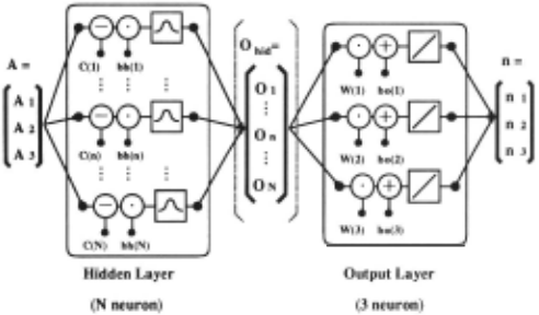
The idea is to use the length of the surface normal, [nt, n2, n3 ], to define a confidence measure. We have found a better idea to be the simultaneous training of a second network, during calibration, to inversely pre­ dict the input, [At, A2, A3] from the estimated output, [nt, n2 , n3]. Comparison between the actual input and the inversely predicted input then serves as a suitable confidence estimate.

The architecture for the two step RBF network is shown in Figure 2. As mentioned, both component net­ works are trained during calibration. During training, each normal vector input to the inverse network neces­ sarily is a unit normal. If the 3D subspace from the calibration sphere is input to this two step network, the output of the second step, which we call the resynthe­ sized input subspace, should be very similar to the origi­ nal input. However, if an impossible triple (i .e., one that could not have arisen from the calibration sphere) is in­ put, we expect the resynthesised input subspace to be quite different since the resynthesized values necessarily correspond to points on the calibration sphere.

3 Illumination Planning

3.1 Implementation

NN-based photometric stereo using more than three light sources can be implemented as follows .

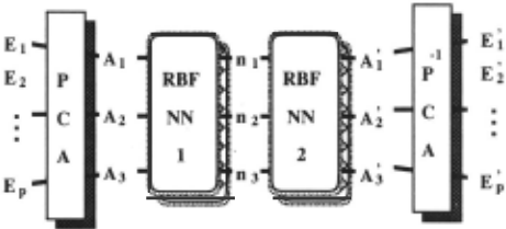
Process consists of two NN units . Two RBF-NNs are learned under the condition that the number of the dimension for both of inputs and outputs is three for each NN. First, PCA gets A = (At, A2, A3) from E = (Et, E2 , · · ·, Ep) to make it efficient to learn the input/output mapping and to save the learning time by NN. Then, A = (At, A2, A3) is input to the first RBF­ NNl and the surface normal vector n=(nt , n2 , n3 ) is ob­ tained, then the inverse RBF-NN2 is applied to estimate A = (At, A2 , A3 ) from n. By applying the inverse trans­ formation of PCA, we can get the corresponding output E= (E~,E~,···,E~).

Confidence estimate for each point on the test object is calculated as

The precision for total points is evaluated as

wh~re Nobj is the total pixel number of the test object reg10n.

Calibration measures reflectance data using an object of known shape. A sphere is a good choice because it is convex, thus eliminating interreflection, because it is easy to dead reckon local surface orientation geometri­ cally from the object silhouette and because it spans all possible visible surface normal vectors. Details of tit~ cal­ ibration procedure used are described elsewhere [Wood­ ham, 1994 ; lwahori et al. , 1995].

Illumination planning is applied by picking up the data that does not give the cast shadow under the multiple light sources for each point on the test object.

3.2 Strategy of illumination planning

Three light source photometric stereo necessarily causes cast shadow problem for the complicated curved object and the image irradiance equation cannot be applied for cast shadow region . Generally, shadow region is given by two causes: one is the region where the shadows de­ pends on the geometrical local shape, and the other is the cast shadow which is defin~d as that anoth~r local shape interrupts the illumination and it casts shadow. Th~ former shadow occurs when the angle between the surfac~ normal v~ctor and the light sourc~ dir~ction v~c­ tor becorn~s greater than 90 degre~s , how~v~r , actual image irradiances still hold some information to r~cover th~ local surface gradient. While, the latter shadow is defined as the cast shadow and it is impossible to use the irradiance values to recover the local surface gradi~nt.

The approach uses the rotational rnultipl~ light sources more than three, and once recovers the distri­ bution of surface orientation for the test object using all light sources. After this process , one can deter­ mine the confidence for each point of the test object from the difference between E = (E1,E2 ,···,Ep) and E' = (E~,E~,···,E;). From the confidence values, th~ method disposes the ill-effected light sources among all light sources and recovers the shape again from only the well-~ffected light sources to get th~ relevant r~sults . This is proposed as the st rategy of th~ illuntination plan­ ning based approach . The procedur~s ar~ giv~n as fol­ lows.

• I . Recovery from all p-light sourc~s
• All p-light sources, i.e., Eall = (E1, E2, · · · , Ep) ar~ input into the NN-units and obtain nail and E~11 .
• Extraction of cast shadow region

The object surface regions can be defined as one of " normal reflection region", " interrefi~ction re­ gion" , "shadows depending on local shape region" and "cast shadow region" . This method finds the "cast shadow region" from the threshold process with Thu to the standard derivation u all of the dif­

• ference of (Eall- E~11 ) for each pixel.

This process can find " normal refiection region" and "shadows depending on local shape region" und~ r tit~

condition that Eall ~ E~11 and CTal/ ~ 0. While, " in­ terrefiect ion region" increases the observed image irradi­ ance and affects to E~11 , but E~ 11 are stable for all light sources and the variance of Call becomes small for this interrefiect ion region.

Only the "cast shadow region" takes the various values for the variance of the difference between Eall and E~ 11 · Then, the values of Call and CTall become high for this "cast shadow region".

From the above reasons, the appropriate threshold process to u all can find the "cast shadow region".

• :3. Disposing light source which casts shadow For each point of the extracted cast shadow region , new combination group sub of light sources is de­ termined by disposing the light source which casts shadow from the all combination of group all using the difference value ThD of each light source.

Let Dall be the difference between Eall and E~11 , then the light source which has the larger value of IDd = IEI­ E{I has the worse one and should be a prior··i disposed as light source which casts shadow .

Since any E{ actually has the positive value for the cast shadow and th~ range of E1 is l ~ss than it and greater than 0 for the same point , only the light sources for which D1 are negative and less than ThD, are disposed.

1. Final recovery for each point without light sources whi ch cast shadow

Image irradiance vector E sub from the illumination of the extracted light source group sub is input into th~ corresponding N N-unit and the shape of cast shadow regions are r~covered again. The vectors ( n .,ub, E~ub) obtained here are used as the final r~­ sults for the cast shadow region .

4 Experiments

4.1 Configuration

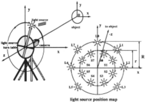
The light source configurations are shown in Figure 3. The distance between object and camera was set to be 200 (em). Fifteen light source directions were used , each differing from the z-axis by 8.58 degrees (i .e., azimuth angle) for the illumination of eight light sources with smaller radius, while by 11.85 degrees for that of seven light sources with larger one.

Two objects are used. One is a pottery sphere, used for calibration purposes, and the other is a pottery moon face. Both objects are made of the same material with the same reflectance properties . No particular assump­ tions for the surface reflectance or light source directions are used or needed for the experiments.

4.2 Construction of NN-Units

This experiments disposes the worst light sources of one to five in the total fifteen light sources. Therefore, the number of NN-units prepared is L.:~~ 1 0 15Cr = 4944 for the combination of ( 15C15 to 15C10) .

The covariance matrix size used to recover the gradient for ~aclt point on the test object depends on the the number of light sources used for each point. The learning count for learning each NN-unit was set to be 40. This value is sufficient for the scale and generalization of N N used in the experiment. The values of th" and thD was set to be 15 and -20 (mean of D) , respectively.

4.3 Results

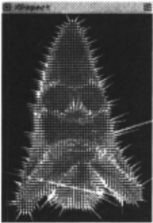
The results of this approach are shown in the Figures 4 to 7. The mean value of the estimated confidence, mean(C), was 4.11619 after the illumination planning, while mean(C) was 4.73629 before applying the illimi­ nation planning.

(b) after illumination planning

Figure 4: Needle maps

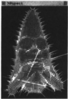
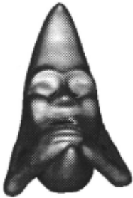
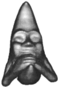
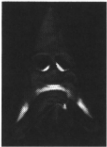
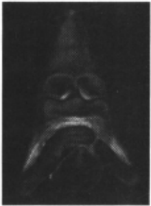
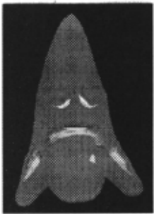
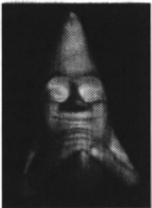
Figure 4 shows the needle map obtained before/after the illumination planning, respectively, while Figure 5 shows the slope map which linearly encodes the slope angle, e, (i.e., the angle between the surface normal and the vector pointing to the viewer) as a gray value in the range black (e = 0) to white (e = -;r/2) . Figure 6 shows the values of the confidence estimate C, encoded as a gray level. Bright values correspond to points in the im­ age where confidence in the estimated surface orientation is lowest. As can be seen, after the illumination plan­ ning, the confidence estimate is apparently improves for the region affected by cast shadows. Figure 7-(a) shows how the region was improved by this illumination plan­ ning as a gray level. Bright values corresponds to the well improved regions . Figure 7-(b) shows an example of the original input images from the light source Ll.

(b) after illumination planning

(b) after illumination planning

Figure 6: Confidence maps

Figure 4-(a) and Figure 5-(a) shows some local ran­ dom results around the two eyes, mouth, and arms, but Figure 4-(b) and Figure 5-(b) improved the results and removed the disconnected vectors around there. Fig­ ure 6-(b) is also improved in comparison with Figure 6-( a) for the corresponding regions. Numerical evalua­ tion shows the mean value of the confidence estimate, mean(C), was improved with the rate of 13.1% and it is shown that the the regions effected by the cast shadow is extracted and sufficiently recovered in addition to the normal regions, and the approach is entirely robust and practical by introducing PCA and neural networks .

(b) An original image of Moon-face : Ll

Figure 7: Reference images

5 Conclusion

This paper proposes a new neural network based pho­ tometric stereo using the illumination planning, a.c; one of the physics based vision approach. The illumination planning determines the cast shadow region and disposes the information of the ill-effected light sources for each point on the object from the output of the neural net­ work.

Shadows depending on local shape has the information to be used for shape recovery but cast shadow cannot be used for photometric stereo. For the implementation , PCA and RBF NN-units are effectively used for the en­ vironment . In the illumination planning, the ill-effected region for each point is found from the output of NN­ units learned for the calibration sphere images from all light sources. One can know which combination of light source is used to get the relevant result for each point. Finally, each combination of NN-units can be applied to recover the surface normal for each point on the test ob­ ject effected by cast shadow. It is valuable to stress that the entire approach is non-parametric, empirical in that no explicit assumptions are made about light source di­ rections or surface reflectance. It is sufficient that the calibration sphere used in training and the subsequent test objects be viewed under the same pattern of illumi­ nation and be made of the same material (i.e, have the same reflectance properties.) The experiment shows the approach is useful and can improve the shape recovery.

As the future subjects, the application of NN to non­ uniform test object, and to the problem of correcting interreflection are remained.

Acknowledgements

Support for the work described in this paper was pro­ vided by the Artificial Intelligence Research Promotion Foundation, Japan. Support for Woodham's research is provided by the Institute for Robotics and Intelligent Systems (IRIS) and by the Natural Sciences and Engi­ neering Research Council of Canada (NSERC) .