Model Minimization, Regression, and Propositional STRIPS Planning

1 Introduction

In this paper, classical planning refers to the proposi­ tional variant of STRIPS planning [Fikes and Nilsson, 1971]. Classical planning is based on a factored represen­ tation for describing planning domains in terms of rules that specify how the dynamic features of the domain {called fluents) change over time. Classical planning problems can be viewed as finite state automata where states correspond to assignments to fluents, the rules compactly encode the state-transition function, and the task is to determine if it is possible to reach some state satisfying the goal from the initial state.

There are well-known algorithms for reducing the size of explicitly represented FSAs by collapsing groups of states that are bisimulation equivalent, i.e., states that behave the same 1 under every action sequence [Hopcroft,

1 Two states behave the same under an action sequence

1971; Paige, 1987]. These automaton minimization algo­ rithms rely, however, on the explicit representation ofthe FSA being minimized. Recent work on model checking in the computer-aided verification community [Burch et al., 1994] has explored the problem of automaton mini­ mization for FSAs represented in factored forms.

Given a classical planning problem, FSA minimiza­ tion techniques compute a (possibly) smaller FSA that captures all the essential information in the problem for­ mulation; we call this FSA the minimal model for the planning problem. The states of the original FSA are partitioned into blocks which constitute the (aggregate) states of the minimal model. This paper explores the rel­ evance for classical planning of the recent model checking work on automaton minimization for factored FSAs.

FSA minimization is in general much more aggressive than classical planning solution techniques. In minimiza­ tion, states are grouped together based on identical be­ havior under all sequences of actions. In contrast, in classical planning solution techniques, we are interested primarily in the goal connectivity and distance to the goal of different states, and are not generally interested in differentiating states based on other variations in be­ havior (e.g., two states that differ only on the basis of action sequences that don't involve goal states may be equivalent for the purpose of planning).

Nevertheless, the algorithms for minimizing a factored FSA bear a significant resemblance to the classical plan­ ning technique of goal regression. 2 The basic step in each algorithm is to find the preimage of a set of states under an action-that is, those states that can reach the given set in one step under the given action. This similarity is the basis for our comparisons.

To assist in our comparisons, we define the new con­ cepts of partial and approximate minimization. A par­ tial minimization of an FSA is a partition of the states of the FSA which is strictly coarser than the minimal partition- that is, a partition that can be refined into the minimized FSA partition. An approximate partial minimization is a partial minization except that in place of the partition of the state space there is a set of pos­ sibly overlapping sets which cover the state space. Re­ gression computes an approximate partial minimization of the planning problem. We also define a systematic re­ gression which computes an exact partial minimization of the planning problem.

if they both reach accept states or both reach reject states under the sequence.

2 Goal regression is just backward chaining search from a goal (or subgoal) representing a set of states.

Both partial and approximate partial minimizations compute partitions that are less refined than the true minimal partition. The approximate partial partition computed by regression makes only those distinctions needed in determining whether the searched action se­ quences can solve the planning problem. We say that such partitions "capture solvability" for the action se­ quences considered- a concept we formalize later on. We also discuss variations of minimization that compute partitions which are more refined than the true minimal partition. These variations can be useful when the re­ sulting partition is easier to compute than the minimal partition, since any computation on the resulting FSA still mimics the original FSA (the drawback being that the size reduction achieved by the minimization may be much smaller than that produced by true minimization). We show how a simple reachability analysis to determine which fluents are irrelevant can also be viewed as an vari­ ant of minimization.

Finally, it is of interest to consider the class of clas­ sical planning problems for which the minimized model is polynomial in the size of the input. In general, the problem of finding a solution to a STRIPS planning problem is PSPACE-complete [Bylander, 1994]. How­ ever, the class of solvable STRIPS planning instances with polynomial-sized models is in NP, as one can sim­ ply guess the polynomial-sized model. We have shown that finding the minimal model is NP-complete under the assumption that it is polynomial in the size of the original STRIPS description.

2 Classical Planning

A classical planning problem is a tuple (X, A, q0 , 9) where X is a set offluents (which for simplicity in exposi­ tion we assume to be boolean state variables), A is a set of actions, q0 is a boolean formula representing the ini­ tial state, and g is a boolean formula representing the set of goal states. If there are m fluents, then there are 2m states corresponding to the set of all possible assignment& to them fluents. We represent individual states and sets of states using boolean formulas, e.g., if X= {A, B, C}, then, depending on the context, A 1\ B 1\ C represents the state in which A, B, and C are assigned true or the set consisting of the same state.

Each action a defines a mapping fa from states to states and is represented as a set of rules of the form l'J -+ <p where the precondition l'J and the postcondition <p are conjunctions of negated and unnegated fluents. The preconditions in an action's set of rules must be mutually exclusive, and variables not determined by the rules remain unchanged. For example, if X= {A, B, C} and a= {A 1\ ·B-+ B 1\ C, A 1\ B-+ ·C}, then !a(AI\

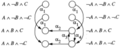
Figure 1: Model for the case in which there are three fluents X = {A, B, C} and four actions: a 1 = { ·B -+ B}, a2 = {B -+A}, a3 = {·A 1\ B 1\ C-+ -.C}, and a4 = { ·A 1\ B 1\ ·C-+ C}.

·BI\C) = (AI\BI\C), fa(AI\BI\C) = (AI\BI\·C), and fa ( ·A 1\ B 1\ C) = ( ·A 1\ B 1\ C). In the remainder of this paper, we restrict our attention to actions represented by a single rule, but our methods apply to the more general case 3 . We define the preimage J;; 1 ( S) of a with respect to a set of states S as

For simplicity here, we consider only the problem of find­ ing any path from the initial state to the goal block. Sim­ ilar issues exist when considering the problem of finding the shortest such path. We consider a planning problem solvable if there exists a path qo, a1, qb ... , an, qn such that fa, (q;_1) = q; for each i, and the goal formula g is true of Qn·

If l'J and <p are a boolean expressions representing sets of states (possibly the same set) and l'J = J;; 1 ( <p), then l'J is said to be a regression of <p with respect to a, and l'J is said to be a subgoal of <p. Since two different for­ mulas can represent the same set, there may be more than one regression for given goal and action. We note that for a 1 :j; a2 the sets corresponding to /;; 1 1 ( <p) and /;;, 1 ( <p) could be equal, disjoint, or different but over­ lapping. In the following, regression step refers to com­ puting the regression of some formula with respect to some action, and regression search refers to any search algorithm that proceeds by performing regression steps on previously computed regression formulas. The term regression graph refers to the graph with nodes corre­ sponding to regression formulas and arcs to the regres­ sion steps (and their associated actions) produced by re­ gression search; we refer to the set of root to leaf paths in this graph as the set of action sequences considered by regression search.

3 Factored Automaton Minimization

In this paper, a state-transition diagram is a graph in which the nodes are sets of states, the arcs are directed, and each arc is labeled with an action. For any given node and action label, there can be only one arc from that node with that action label. Note that such a di­ agram describes a deterministic finite state automaton. We use the term "model" for a state transition diagram that captures the dynamics of a planning problem:

3 Simple regression for the more general case requires the manipulation of general boolean formulas , and thus the sys­ tematic regression we introduce later may compare more fa­ vorably to simple regression when the actions are complex in this way.

Definition 1 We say that a state-transition diagram is a model for a classical planning problem if

1. the nodes form a partition of the planning state space, and
2. for any state q, node v1 containing q, node v2 , and action a,
3. (a) fa ( q) is in Vz if there is an arc from Vt to Vz labelled a, and
4. (b} f a ( q) is in Vz only if there is an arc from v1 to Vz labelled a.

If conditions 1 and 2{a) hold without condition 2(b) we say that the diagram is a partial model. If condition 1 is additionally relaxed to merely require the nodes to . cover the state space (but perhaps overlap), we say that the diagram is an approximate partial model (sometimes abbreviated "approximate model").

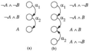
Note that there can be more than one model for a given planning problem, corresponding to different partitions of the domain, though in general most partitions can­ not be used to define a model. Every model·of a prob­ lem contains all the information in the original problem: models smaller than the original problem can be viewed as compact forms of the original problem. It is a theorem that for every problem there exists a minimal model-a model with a partition P such that every other model uses a refinement of P. Figure 1 depicts the model for a particular planning instance with a degenerate parti­ tion consisting of singleton blocks, and Figure 2(a) shows the minimal model for the same problem. Reachability queries on the minimal model have the same answers as those on the original model.

We note that every model is associated with a par­ tition of the state space-that partition formed by the nodes of the model. Similarly, any partition induces at most one model (some partitions cannot be used to form models). We will be somewhat free in referring to models as partitions. We also use a particular partial order on partitions (and hence on models): we say that a parti­ tion P1 is coarser than a partition P2 if P1 can be refined into Pz- and we say that Pz is finer than P1·

A partial model is a diagram in which every arc is "cor­ rect" (i.e., corresponds correctly to the planning prob­ lem) but may have missing arcs as well as blocks which need to be refined. We call a partial model generic for a planning problem if it is coarser than the minimal model for that problem, so that further refinement could gen­ erate the full minimal model. The minimization pro­ cess described below computes a series of generic partial models leading eventually to the minimal model. An approximate partial model is additionally allowed to be undecided about which block certain states will fall into (by having blocks overlap). An approximate model can always be converted into a partial model by disambiguat­ ing the overlaps- i.e., shrinking blocks until they are disjoint. If an approximate model can be so converted into a generic partial model, we also call the approximate model generic.

The Model Minimization Algorithm. Let B and C be blocks of partition P and let a be any action. We define the SPLIT operation as follows

where P' is P with C replaced by 4 C' and C" defined by

Lee and Yannakakis [1992) describe a model minimiza­ tion algorithm which uses the SPLIT operation to com­ pute the minimal model for an FSA in factored form. In its application to planning, the algorithm begins with an initial partition Po consisting of two blocks, those states that satisfy the goal and those that don't. The algorithm then repeatedly chooses some B, C, and a and computes a refined partition Pi+! = SPLIT(B, C, P;, a). When no additional refinement is possible, the resulting partition induces the minimal model of the problem. This algo­ rithm calls SPLIT polynomially many times in the size (number of blocks) of the final partition. If we want to compute the most compact representation of each block in the partitition, then SPLIT is NP-hard.

Several variations on model minimization are rele­ vant for this work. First, Lee and Yannakakis de­ scribe a variant we will call reachable model minimiza­ tion which computes a model that is minimal for the states reachable from the initial state, but arbitrary for other states-space precludes making this notion more formal here. Second, it is possible to replace the SPLIT operation with operations that do more split­ ting than SPLIT 5 . We call a block-splitting operation SPLIT'(B,C,P,a) adequate if it produces a partition of C that refines SPLIT(B, C, P, a). Performing model minimization with an adequate splitting operation pro­ duces a (possibly reduced) model which is not necessarily minimal. Figure 2(b) shows a reduced model generated using an adequate but nonoptimal splitting operation, FSPLIT, which we define later.

Complexity of Minimization. There are planning problems for which the shortest solution is exponentially long in the length of the problem description [Bylander, 1994). This fact directly implies that there are problems with exponentially large minimal models, and therefore that minimization must take at least exponential time. However, one might hope that in those cases where the minimal model is "small", minimization could find it quickly. Unfortunately, by a reduction from SAT, we are able to show that even when the minimal model is polynomial in size, minimization is NP-hard.

4 If either C' or C" is empty, then SPLIT( B, C, P, cr) = P. 5 Such operations may be more efficient, as we discuss be­ low, which is why we would do this.

-.A/\--,B B ..

Theorem 1 Given a bound and a planning problem whose minimal model is polynomial in size, the problem of determining whether there exists a model of size no more than the bound is NP-complete.

4 Regression

In this section, we argue that classical regression com­ putes an approximate partial model of the planning problem. But regression doesn't compute just any par­ tial model- it computes a partial model capturing cer­ tain useful information 6 · We say that a partial model captures solvability for an action sequence if every path that achieves the goal with that action sequence is rep­ resented in the model:

Definition 2 A partial model captures solvability for action sequence a1···ak if every path qlat···ak-lqk such that qk achieves the goal has a corresponding path v1a 1 · · ·ak-IVk in the model such that each q; is in block v;.

We say that an approximate partial model captures solv­ ability for an action sequence if it can be disambiguated into a partial model which does. We also refer to cap­ turing solvability for a set of action sequences, meaning capturing solvability for each sequence in the set.

The key to understanding regression as minimization lies in thinking of the sub goals generated by regression as representing sets of states (those states that satisfy the subgoal). Each such set of states shares a simple prop­ erty: it is the set of all states which can reach the goal under a particular action sequence (the reverse of the sequence of actions under which the goal was regressed to get that subgoal). A regression search tries different action sequences, for each one generating a su bgoal cor­ responding to the set of states which achieve the goal under that sequence. Each new subgoal/set of states is generated by a regression step from a previous sub­ goal/set of states. If a subgoal is ever true of the initial state, then the search terminates.

Note that different subgoals could be true of the same single state-i.e., the sets of states described could overlap. The sets of states corresponding to the subgoals can be viewed as nodes in an approximate partial model , where the regression steps which generated the states correspond to arcs in the model. Because the subgoals may overlap, the partial model is approximate, but each regression step locally preserves the fact that the dia­ gram being constructed is a generic partial model which captures solvability for the action sequences which have been regressed. The following theorem can be proven by induction on the number of regression steps taken.

6Every planning problem admits the trivial partial model built from the trivial partition into singleton sets with no arcs, as well as the trivial partial model built from the goal/non-goal partition, again with no arcs.

Theorem 2 At any point, the regression graph is a generic approximate partial model which captures solv­ ability for the action sequences considered by the regression search to that point. ·

The model minimization algorithm described in the previous section also takes simple local steps (analogous to regression steps) using the SPLIT operation to con­ struct .sets of states which behave uniformly under se­ lected action sequences. At the completion of minimiza­ tion, the blocks of the resulting partition correspond to sets of states which behave the same under all action sequences. But along the way, the partition constructed at each step forms a partial model in which states in the same block behave the same only for selected action se­ quences. Just as regression search involves a search strat­ egy to select which regression to do next, model mini­ mization must also select which SPLIT step to do next­ in each case extending the set of action sequences which have been explored. Minimization strategies which al­ ways split the block containing the initial state corre­ spond closely to regression strategies. 7

The central distinction between simple regression and minimization is that minimization constructs a series of generic partial models whereas regression constructs a series of generic approximate partial models. The regres­ sion subgoals may overlap considerably, whereas mini­ mization at all times maintains a partition. For some problems, this difference illuminates a potential ineffi­ ciency in regression- the same state can be "regressed" many times under the aegis of different but overlapping subgoals. We introduce a variant of regression which we call systematic regression to eliminate this difference.

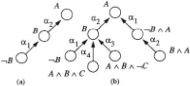
In systematic regression, each subgoal must be disjoint from all previous subgoals. In order to achieve this, the regression search must maintain a boolean formula de­ scribing the set of states which have not yet been covered by a subgoal 8 · Each new subgoal must be conjoined with this boolean formula to ensure its disjointness with previ­ ous subgoals. Just as in simple regression, a search strat­ egy controls the order of the regression steps takensystematic regression differs from simple regression only in that the individual regression steps are modified to maintain the disjointness of the subgoals generated. Fig­ ure 3 shows the regression graphs generated by both sys­ tematic and simple regression for the example problem shown in earlier figures.

7 The reachable model minimization algorithm referred to in the previous section does exactly this- in its efforts to construct a minimized reachable model it will split only the block containing the initial state.

8 This set of states corresponds to the block containing the initial state during minimization, and can also be viewed as the set of states which have not yet been found goal­ connected by regression.

Theorem 3 The regression graph generated by system­ atic regression at any point is a generic partial model which captures solvability for the action sequences con­ sidered by the regression search to that point.

If the boolean formula for a subgoal is unsatisfiable, systematic regression must stop searching below that subgoal-it is this pruning that reduces the number of subgoals generated compared to simple regression. For some problems, systematic regression will generate ex­ ponentially· fewer subgoals than simple regression, due to the elimination of overlap. For an example of this phenomenon, consider a planning problem with n stages where at each stage there are two choices of action se­ quence which result in the same state in the next stage (via different paths). Minimization will construct O(n) blocks on such a problem, but regression will construct 0(2n) subgoals. Unfortunately, systematic regression depends on an unsatisfiability test at each node which is NP-hard; in practice the usefulness of systematic regres­ sion will be limited to those cases where there is sub­ stantial overlap between subgoals (i.e., many different action sequences have similar effects) and will depend on the ~rowing efficiency of the best known satisfiability testers lSelman et al., 1992].

Theorem 4 Unlike simple regression, systematic re­ gression never generates more subgoals than there are blocks in the minimal model.

5 Reachability Analysis

Computing the minimal model for a planning problem relies critically on the SPLIT operation, which we've in­ dicated can have exponential cost. One way around this problem is to compute instead a refinement of the min­ imal model by using a variant of SPLIT which is less expensive and does at least as much block splitting. 9

9 Allowing excess splitting can be cheaper because it re­ lieves the splitting operation of the task of deciding whether

Such a refined model has many of the same advantages of the minimal model: reachability in the refined model still captures reachability in the original problem, for in­ stance. The disadvantage to computing an overly refined model is that the model may have many more states than the truly minimal model, giving up the advantage of reduced size that was originally sought. Neverthe­ less, there are problems for which a significant problem size reduction can be gained using an adequate but non­ optimal split operation.

To guarantee that the resulting model is a refinement of the minimal model, the splitting operation used must be adequate: it must do at least as much splitting as SPLIT would have done. The option to do extra split­ ting allows us to consider using a representation for par­ titions which cannot represent every partition: if a split is called for which we cannot represent, we can always perform additional splitting to get a representable parti­ tion (the representation must have at least this property, though). One such partition representation is what we call a fluentwise partition representation. Given a set of fluents xl, consider the partition of the state space where two states are in the same block exactly when they agree on the values of the variables in X1 . We call any partition which can be represented in this manner a fluentwise partition. Note that most partitions of the state space are not fluentwise partitions.

We now define an adequate split operation FSPLIT for manipulating fluentwise partitions. Given fluentwise partition P, blocks B and C from P, and action a, we define FSPLIT(B, C, P, a) to be the coarsest fluen­ twise refinement of SPLIT(B, C, P, a). FSPLIT is easily computed in time linear in the size of its inputs. Using FSPLIT in place of SPLIT, the model minimization algo­ rithm can find a (possibly) reduced model which refines the minimal model in time polynomial in the original problem size. 10 The model found may of course have exponentially more states the minimal model. A model found by FSPLIT minimization is given in Figure 2(b).

FSPLIT minimization is a minimization-oriented de­ scription of a familiar and simple reachability analysis which can be used to simplify propositional planning problems. Specifically, a simple transitive closure can de­ termine the set of fluents relevant to the problem, which is the least set P of fluents containing every fluent which appears in the goal description and every fluent which appears in the precondition for some action rule whose postcondition contains a fluent in P. The set of rele­ vant fluents can easily be computed in polynomial time. Once this set is computed, the problem can be reduced by removing the irrelevant fluents along with any actions whose rules mention them. The resulting state space is exactly the blocks of the partition found by FSPLIT

to split-the most trivial variant of SPLIT would just split fully into a partition of singleton sets.

10 Note that the ftuentwise partition representation is an implicit representation; the final partition can have exponen­ tially many blocks but can still be constructed in polynomial time.

minimization.

6 Related Work

Burch et al. [1994] is the standard reference on sym­ bolic model checking for computer-aided design. Our algorithms and analyses were primarily motivated by the work of Lee and Yannakakis [1992] and Bouajjani et al. [1992]. Backstrom and Klein [1991], Bylander [1994], and Gupta and Nau [1991] provide basic results con­ cerning the complexity of STRIPS planning and special cases. Etzioni [1993] describes a particular algorithm for reachability analysis and provides a survey of related techniques.

In [Dean and Givan, 1997] we show how model min­ imization can be used to solve implicit (or factored) Markov decision processes (MDPs) with very large state spaces, and prove that our model minimization based al­ gorithms are asymptotically equivalent to existing meth­ ods (e.g., [Boutilier et al., 1995]) that operate on implicit MDPs. In [Dean et a/., 1997] we show how model reduc­ tion techniques can be used to trade time for space in computing approximately optimal solutions to Markov decision processes. Finally, in the longer version of this paper, we show how the methods of this paper can be used to understand the advantages of the explanation­ based reinforcement learning algorithm developed by Di­ etterich and Flann [1995].

7 Conclusions

In this paper, we demonstrate how traditional meth­ ods for solving propositional STRIPS planning prob­ lems can be viewed in terms of finite automata (model) minimization. Given a finite automaton whose state­ transition function is defined by a set of STRIPS rules, we show how regression search and simple reachability analysis can be viewed as methods for constructing a finite automaton of reduced size. We also show how existing model minimization methods can be applied to solve propositional planning problems and determine that solving such problems in the case in which the min­ imal model is polynomial in the size of the input is NP­ complete.

It should be noted that there are potential pitfalls in extrapolating from recent success in computer aided ver­ ification using model minimization techniques to possi­ ble gains in tackling STRIPS problems. The verification problems were rendered easier in part due to symme­ tries in hardware and software that result in significant aggregation in the state space. Similar sorts of symme­ try may exist in some factory domains but whether or not the resulting reductions are enough to render the problems tractable remains to be seen.