
Extracting Propositions from Trained Neural Networks
Proceedings of the Fifteenth International Joint Conference on Artificial Intelligence. Neural Networks. Pages 1098-1104.
© 1997 International Joint Conferences on Artificial Intelligence
Abstract
This paper presents an algorithm for extracting propositions from trained neural networks. The algorithm is a decompositional approach which can be applied to any neural network whose output function is monotone such as sigmoid function. Therefore, the algorithm can be applied to multi-layer neural networks, recurrent neural networks and so on. The algorithm does not depend on training methods. The algorithm is polynomial in computational complexity. The basic idea is that the units of neural networks are approximated by Boolean functions. But the computational complexity of the approximation is exponential, so a polynomial algorithm is presented. The authors have applied the algorithm to several problems to extract understandable and accurate propositions. This paper shows the results for votes data and mushroom data. The algorithm is extended to the continuous domain, where extracted propositions are continuous Boolean functions. Roughly speaking, the representation by continuous Boolean functions means the representation using conjunction, disjunction, direct proportion and reverse proportion. This paper shows the results for iris data.
- R. Andrews, J. Diederich and A.B. Tickle: Survey and critique of techniques for extracting rules from trained artificial neural networks, Knowledge-Based Systems, Vol.8, No. 6, pp.373-189, 1995.
- M.W. Craven and J.W. Shavlik: Learning symbolic rules using artificial neural networks, Proceedings of the Tenth International Machine Learning Confer- ence, pp. 73-80,1993.
- M. Ishikawa: Structural Learning with Forgetting, NEURAL NETWORKS, Vol.9, No.3, pp.509-521, 1996.
- N. Linial, Y. Mansour and N. Nisan: Constant Depth Circuits, Fourier Transform, and Learnabil- ity, Journal of the ACM, Vol.40, No.3, pp.607-620, 1993.
- J.R. Quinlan: C4.5: Programs for machine learn- ing, Morgan Kaufmann Pub., 1993.
- J .W. Shavlik: Combining Symbolic and Neural Learning, Machine Learning, 14, pp.321-331, 1994.
- H. Tsukimoto and C. Morita: The discovery of propositions in noisy data, Machine Intelligence 13, pp.143-167, Oxford University Press, 1994 .
- H. Tsukimoto: The discovery oflogical propositions in numerical data, AAAI'94 Workshop on Knowl- edge Discovery in Databases, pp.205-216, 1994.
- H. Tsukimoto: On continuously valued logical func- tions satisfying all axioms of classical logic, Systems and Computers in Japan,Vol.25, No.12, pp.33-41, SCRIPTA TECHNICA, INC., 1994.
- H. Tsukimoto and C. Morita: Efficient algorithms for inductive learning-An application of multi-linear functions to inductive learning, Machine Intelli- gence 14, pp.427-449, Oxford University Press, 1995.
References were extracted automatically from the PDF and may contain errors.
Full text extracted automatically from the PDF; figures, tables and equations may differ. The PDF is the version of record.
1 Introduction
Extracting rules or propositions from trained neura: net works is important[!], [6]. Although several algonthms have been proposed by Shavlik, Ishikawa and others [2],[3], every algorithm is subject to problems in that it is applicable only to certain types of networks or to certain training methods.
This paper presents an algorithm for extracti~g pro?o sitions from trained neural networks. The algonthm 1s a decompositional approach which can be applied to any neural network whose output function is monotone such as sigmoid function. Therefore, the algorithm can be applied to multi-layer neural networks, recurrent neural networks and so on. The algorithm does not depend on training methods, although some other methods[2],
[3] do. The algorithm does not modify the training re sults, although some other methods [2] do. Extracted propositions are Boolean functions. The algorithm is polynomial in computational complexity.
The basic idea is that the units of neural networks are approximated by Boolean functions. But the computa tional complexity of the approximation is exponential, so a polynomial algorithm is presented. The basic idea of reducing the computational complexity to a polynomial is that only low order terms are generated, that is, high order terms are neglected. Because high order terms are not informative, the approximation by low order terms is accurate[4].
In order to obtain accurate propositions, when the hidden units of neural networks are approximated to Boolean functions, the distances between the units and the functions are not measured in the whole domain, but in the domain of learning data. In order to obtain simple propositions, only the weight parameters whose absolute values are big are used.
The authors have applied the algorithm to several problems to extract understandable and accurate propo sitions. This paper shows the results for votes data and mushroom data.
The algorithm is extended to the continuous domain, where extracted propositions are continuous Boolean functions. Roughly speaking, the representation by con tinuous Boolean functions means the representation us ing conjunction, disjunction, direct proportion and re verse proportion. This paper shows the results for iris data.
Section 2 explains the basic method. Section 3 presents a polynomial algorithm. Section 4 describes the experiments. Section 5 extends the algorithm to contin uous domains and applies it to iris data.
The following notations are used. x, y, .. stand for vari ables. j, g, .. stand for functions.
2 The basic method
There are two kinds of domains, that is, discrete domains and continuous domains. The discrete domains can be reduced to {0, 1} domains by dummy variables. So on~y {0, 1} domains have to be discussed. Here, the domam is { 0, 1}. Continuous domains will be discussed later.
2.1 The basic method
The basic method is that the units of neural networks are approximated by Boolean functions. The output func tions are sigmoid functions, so the values of the units are [0,1].
Let (li) be the values of a unit of a neural network. Let (g;)(g; = 0 or 1) be the values of Boolean functions. The basic method is as follows:
This method minimizes Euclidean distance.
Fig. 1 shows a case of two variables. Crosses stand for the values of a unit of a neural network and circles stand for the values of a Boolean function. 00, 01, 10 and 11 stand for the domains, for example, 00 stands for X= O, y = 0.
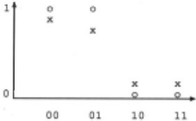
In this case, the values of the Boolean function g(x,y) are as follows:
Generally, let g(xl> ... , Xn) stand for a Boolean function, and let g;(i = 1, .. . , 2n) stand for values of a Boolean function, then the Boolean function is represented by the following formula:
where "2::: is disjunction, and a; is the atom corresponding to g;, that is,
where
where IT stands for conjunction, x stands for the nega tion of x, and e; is the substitution for x;, that is, e; = 0 or 1. The above formula can be easily verified. There fore, in the case of Fig. 1, the Boolean function is as follows:
2.2 An example
We show that the proposition of Exclusive OR, that is, xyVxy, can be obtained by approximating a neural net work which has learned Exclusive OR using the back propagation method. First, we explain the structure of the network. Second, we analyze the learning results.
Fig. 2 shows the structure of the neural network.
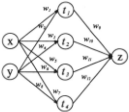
In Fig. 2, x and y are inputs, z is an output, and t;'s are the outputs of four hidden units. Each output is represented as follows:
t1 = 8(w1x + w2y + h1),
t2 = 8(w3x + w4y + h2),
t3 = 8(wsx + woy + h3),
t4 = 8(w7x + wsy + h4),
where w;'s stand for weight parameters, 8(x) stands for sigmoid function and h; 's stand for biases.
The learning results with 1000 time repetition are as follows:
w1 = 2.51, w2 = -4.80, w3 = -4.90,
w4 = 2.83, w5 = -4.43, w6 = -4.32,
W7 = -0. 70, Ws = -0.62, Wg = 5.22,
w1o = 5.24, w11 = -4.88, w12 = 0.31,
h4 = -0.85, h5 = -2.19.
hl = -0.83, h2 = -1.12, h3 = 0.93,
For example,
t1 = 8(2.51x - 4.80y - 0.83),
and the values of t1 (0, 0), t1 (0, 1), t1 (1, 0), and t1 (1, 1) are as follows:
t1 (1, 1) = 8(2.51 · 1- 4.80 · 1- 0.83) = 8( -3.12),
tl (1, 0) = 8(2.51 . 1 - 4.80 . 0- 0.83) = 8(1.68),
t1 (0, 1) = 8(2.51 · 0- 4.80 · 1- 0.83) = 8( -5.63),
8( -3.12) ~ 0, 8(1.68) ~ 1, 8( -5.63) ~ 0, and 8( -0.83) ~ 0, therefore
t1 (0, 0) = 8(2.51 · 0 - 4.80 · 0 - 0.83) = 8( -0.83).
t1 ~ xy.
In a similar manner, the others are approximated by the following Boolean functions:
t2 = xy,
t3 = xy,
t4 = 0.
The learning result of z is as follows:
z = tlt2 v tlt2t3 v ttf2t3.
By substituting t1 = xy, t2 = xy, and t3 = xy, in the above formula,
z = xyVxy
has been obtained. This proposition is Exclusive OR.
Now we have confirmed that the logical proposition of Exclusive OR can be obtained by approximating the neural network which has learned Exclusive OR. We un derstand the following items.
- The learning results of 4 hidden units and an output unit.
- The output of hidden unit 4, t4 , is not included in the Boolean function of the output unit, z, so hidden unit 4 does not work and can be deleted.
- The other three hidden units work, so they are nec essary and cannot be deleted.
A merit of the decompositional approach is that trained neural networks can be understood by the unit.
3 A polynomial algorithm
Obviously, the computational complexity of the basic method is exponential, so the basic method is not re alistic. Therefore, the computational complexity should be reduced to a polynomial. This section presents the polynomial algorithm. The basic idea of reducing the computational complexity to a polynomial is that DNF formulas consisting of only low order terms are gener ated from the lowest order up to a certain order, that is, high order terms are ne~lected. Because high order terms are not informative[4J, the approximation by low order terms is accurate.
The brief outline of the algorithm follows.
- Check the existences of terms after the approxima tion from the lowest order.
- Connect the terms which exist after the approxima tion to make a DNF formula.
- Execute the above two procedures up to a certain order.
In this section, first, the condition that a term x; 1 · ·X;kx;H 1 ··X; 1 exists in the Boolean function after approx imation is presented. Second, the generation of DNF formulas is explained. Third, in order to obtain accu rate propositions, the condition is modified in a manner such that the distance between the hidden unit of a neu ral network and a Boolean function is not measured in the whole domain, but in the domain of the learning data. Fourth, in order to obtain simple propositions, the condition is modified in a way such that only the terms consisting of variables whose weight parameters' absolute values are big are generated.
3.1 The condition that Xi 1 · ·XikXik+l · ·Xi1 exists in the Boolean function after approximation
Let a unit of a neural network be
where SO is an arbitrary function. Let the orthonormal expansion be
where "+" and "·" are the sum and the product of ele mentary algebra and x is 1- x. Boolean functions can be represented by elementary algebra and the atoms can be the orthonormal functions. Due to space limitations, for details, see [10].
Proof h can be obtained by substituting x1 = · · · = Xn = 1 in the following formula:
f2 .. can be obtained by substituting x1 = · · · = Xn = 0 in the above formula. The other coefficients can be obtained in a similar p1anner. D
Theorem 2 The condition that
exists in the Boolean function after approximation is as follows:
where SO means a monotone increasing function.
Proof Consider the existence condition of x1 in the Boolean function after approximation. For simplifica tion, this condition is called the existence condition. Be cause
the existence of x1 equals the existence of the following terms:
The existence of the above terms means that all coeffi cients of these terms JI, h, ... , f2n-1 are greater than or equal to 0.5 (See 2.1). That is, the existence condition lS
each !;(1 :::;; i :::;; 2n-l) contains p1. If each Pi is non negative, f 2n-t(= S(pl +Pn+I)) is the minimum because the other j;'s contain other pj's, and therefore the other fi's are greater than or equal to f2n-t(= S(p1 + Pn+l)). Note that the above argument holds, because S(-) is monotone increasing. Generally, since each Pi is not nec essarily non-negative, the min{!;} is /; which contains all negative Pi· That is,
which necessarily exists in /;(1 :::;; i :::;; 2n-l ), because fi(1 :::;; i :::;; 2n-l) is
From the above arguments, the existence condition of x1, min{/;}~ 0.5, is as follows:
Since S(p1x1 + ... + PnXn + Pn+I) is symmetric for x;, the above formula holds for other variables; that is, the existence condition of x; is
Similar discussions hold for x;, so we have the following formula:
Similar discussions hold for higher order terms x; 1 · ·x;~x;~+t ··'X;" so we have the following formula:
0
Since the output function is monotone increasing, this theorem cannot be applied to units whose output func tion is a Gaussian function. Moreover, it can be easily verified that a similar theorem holds when the output function is monotone decreasing.
3.2 Generation of DNF formulas
The algorithm generates terms using (1) from the low est order up to a certain order. A DNF formula can be generated by taking the disjunction of the terms gen erated by (1). · A term whose existence has been con firmed does not need to be re-checked in higher order terms. For example, if the existence of x is confirmed, then it also implies the existence of xy, xz , ... , because x = x V xy V xz V ... ; hence, it is unnecessary to check the existence of xy, xz, .... As can be seen from the above discussion, the generation method of DNF formulas in cludes reductions such as xy V xz = x. An example follows. Let
be a unit of a neural network. For x;(i = 1, 2, 3, 4, 5),
and therefore x1 exists. For x;xi(i,j = 2,3,4,5),
and therefore no x;x i exists. For x;xjxk(i,j,k = 2,3,4,5),
and therefore x2x3x4 exists. Because higher order terms cannot be generated from x5, the algorithm stops. Therefore, x1 and x2x3x4 exist and the DNF formula is the disjunction of these terms, that is, x1 V x2x3x4.
3.3 A modified condition
This subsection discusses the improvement of the accu racy of the proposition obtained from a hidden unit. In the domain outside the domain of the learning data, the values of a trained neural network are predicted values. So the values in the domain are not reliable. If we have a trained network and no learning data, we cannot know which is the domain of the learning data. Thus only (1) is available. If we have a trained network and the learning data, we can use the domain of the learning data in order to improve the accuracies of the propositions obtained. In order to obtain accurate propositions, when the units of neural networks are approximated to Boolean func tions, the distances between the units and the functions are not measured in the whole domain, but only in the domain of the learning data. That is, the left-hand side of (1), which means the minimum value for a term over the whole domain, is modified to the minimum value for a term in the domain of the learning data. Theorem 2 is modified as shown below.
Theorem 3 Let a unit of a neural network be
then, the existence condition of a term
after the approximation is as follows:
where ei is 0 or 1 and S(-) means a monotone increasing function. The domain used for calculating the minimum value in the above formula is limited to the domain of the learning data.
For example, let three attributes of a learning data be ( x1, x2, X3) and the attribute values be binary. Assume that the learning data are in the table below.
| data | XI | X2 | XJ | class |
|---|---|---|---|---|
| 1 | 0 | 0 | 1 | 0 |
| 2 | 1 | 0 | 0 | 0 |
| 3 | 1 | 1 | 0 | 1 |
In this case, the domain of the learning data is (0, 0, 0), (1, 0, 0) and (1, 1, 0), and a unit of a neural net work is
The existence condition of XI after the approximation is as follows:
But, the checking range is limited to the domain of the learning data, so the checking range is limited to the domain of the data 2 and data 3 where xi = 1. Therefore the existence condition is as follows:
Of course, this modified condition is not applied to the output units in 3-layer networks, because the inputs of the output units come from the hidden units. Therefore, (1) is applied to the output units.
3.4 Weight parameters
Let's sort weight parameters p;'s as follows:
When terms are generated, if all weight parameters are used, the propositions obtained are complicated. There fore unimportant parameters should be neglected. In this paper, p;'s whose absolute value is small are re garded as the unimportant parameters. We will use p;'s up to a certain number, that is, we neglect small p;'s.
How many weight parameters are used is the next problem. Here, the weight parameters PI>···,Pk are used, where k is determined by a value based on Fourier trans form of logical functions[4]. Due to space limitations, the explanation is omitted, which will be presented in another paper.
3.5 Computational complexity of the algorithm and error analysis
The computational complexity of generating the mth or der terms is a polynomial of nCm, that is, a polynomial of n. Therefore, the computational complexity of gen erating DNF formulas from neural networks is a poly nomial of n. Usual generations will be terminated up to a low order, because understandable propositions are desired. Therefore, the computational complexity is usu ally a polynomial of a low order.
In the case of the domain {0, 1}, Linial showed the following formula [4]:
where f is a Boolean function, S is a term, lSI is the order of S, k is any integer, ](S) denotes the Fourier transform of f at S and M is the circuit's size of the function. The above formula shows the high order terms have little power; that is, low order terms are informa tive. Therefore, a good approximation can be obtained by generating up to a certain order.
3.6 Comparisons
This subsection briefly compares the algorithm with other algorithms. Algorithms may be evaluated in terms of five aspects: expression form, internal struc ture, network type and training method, quality, com putational complexity[!]. Here, comparisons focus on internal structure, training method and network type.
internal structure : There are two techniques, namely decompositional and pedagogical. The de compositional algorithms obtain rules by the unit and aggregate them to a rule for the network. The pedagogical algorithms generate examples from the trained network and obtain rules from the examples. Obviously, the decompositional algorithms are bet ter than the pedagogical algorithms in understand ing the internal structures. Therefore, for example, the decompositional algorithms can be also used for the training control.
training method : The algorithm does not depend on training methods, although some other methods do. For example, [2] and [3] use special training methods and their algorithms cannot be applied to networks trained by the back-propagation method. The algo rithm does not modify the training results, although some other methods [2] do.
network type : The algorithm does not depend on net work types, although some other methods do. For example, [2] cannot be applied to recurrent neural networks.
4 Experiments
The training method is the back-propagation method. The repetition is stopped when the error is less than 0.01. Therefore, the error after the training is less than 0.01. The data used for the training are also used for the prediction. Therefore, the accuracy of the trained neural networks is 100%. Usual prediction experiments use data different from those used for the training. But, in this case, it is desired that the accuracy of neural networks be 100%, because we want to see how Boolean functions can approximate the neural networks. Generating terms of propositions are terminated up to second order, because simple propositions are desired.
4.1 votes data
This data consists of the voting records of the U.S. House of Representatives in 1984. There are 16 binary at tributes. Classes are Democrat and Republican. The number of samples used for the experiment is 232. The accuracies of propositions extracted from the trained neural networks are shown in the table below. In the table, i.w.p. stands for initial weight parameter and the numbers in the column of hidden layer mean the num bers of hidden units.
| hidden layer | i.w.p.1 | i.w.p.2 | i.w.p.3 |
| 0 | 0.974 | 0.974 | 0.974 |
| 3 | 0.983 | 0.970 | 0.978 |
| 4 | 0.978 | 0.974 | 0.974 |
In the case of 3 hidden units and i.w.p.1, the following propositions have been obtained:
Democrat: (physician-fee-freeze:n) V (adoption-of-the budget-resol u tion:y) (anti-satellite-test-ban:n) (synfuels corporation-cutback:y ),
Republican: (physician-fee-freeze:y) ( (adoptionof-the-budget-resolution:n) V (anti-satellite-test-ban:y )V (synfuels-corporation-cutback:n) ).
In the other cases, similar results have been obtained. The results for votes data by C4.5[5], which is a typical algorithm for machine learning, are as follows:
(physician-fee-freeze:n) V (adoption-of-the budget-resolution:y) (synfuels-corporation-cut back:y) -+ Democrat,
(adoption-of-the-budget-resol ution:n) (physician-fee freeze:y) V (physician-fee-freeze:y )(synfuels-corporation cutback:n) -+ Republican.
The accuracy of the result ofC4.5 is 97.0%, so the propo sitions extracted from trained neural networks by the al gorithm are a little better than the results of C4.5 in accuracy and almost the same as the results of C4.5 in understandability. ·
4.2 mushroom data
There are 22 discrete attributes concerning mushrooms such as the cap-shapes. Classes are edible or poisonous. The number of samples is 4062. The accuracies of propo sitions extracted from the trained neural networks are shown in the table below.
| hidden layer | l.w.p.1 | l.w.p.2 | l.w.p.3 |
|---|---|---|---|
| 0 | 0.930 | 0.973 | 0.985 |
| 3 | 0.956 | 0.983 | 0.959 |
| 4 | 0.961 | 0.952 | 0.985 |
In the case of 3 hidden units and i .w.p.1, the following propositions have been obtained:
edible: (gill-size: broad) ( (odor: almond) V (odor: anise) V (odor: none)), poisonous: (gill-size: narrow) V..., (odor: almond) -.(odor:anise) -.(odor:none).
In the other cases, similar results have been obtained. The results for mushroom data by C4.5 are as follows:
(odor: none) V (odor: almond) V (odor: anise) -+ edible,
(odor:foul) V (odor:spicy) V (odor:fishy) V (odor: pungent) V (odor: creosote) -+ poisonous.
The accuracy of the result of C4.5 is 98. 7%, so the propo sitions extracted from trained neural networks by the algorithm are a little worse than the results of C4.5 in accuracy and almost the same as the results of C4.5 in understandability.
5 Extension to the continuous domain
5.1 The basic idea
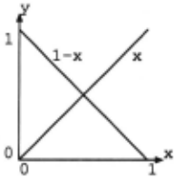
In this section, the algorithm is extended to continu ous domains. Continuous domains can be normalized to f 0,1l domains by some normalization method. So only 0,1 domains have to be discussed. First, we have to present a system of qualitative expressions correspond ing to Boolean functions, in the (0,1] domain. The au thor presents the expression system generated by direct proportion, reverse proportion, conjunction and disjunc tion. Fig.3 shows the direct proportion and the inverse proportion. The inverse proportion (y = 1 - x) is a little different from the conventional one (y = -x ), because y = 1 - x is the natural extension of the negation in Boolean functions. The conjunction and disjunction will be also obtained by a natural extension. The functions generated by direct proportion, reverse proportion, con junction and disjunction are called continuous Boolean functions, because they satisfy the axioms of Boolean algebra.
Since it is desired that a qualitative expression be ob tained, some quantitative values should be ignored. For example, two functions "A" and "B" in Fig. 4 are differ ent from direct proportion x but the two functions are proportions. So the three functions should be identified as the same one in the qualitative expression. That is, in
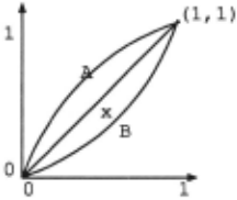
[0,1], xk(k ;::: 2) should be identified with x in the qual itative expression. Mathematically, a norm is necessary, by which the distance among the three functions is 0. The qualitative norm can be introduced.
In {0,1 }, a unit of a neural network is a function f : {0, 1} --+ R. In {0,1}, xk = x, because ok = 0 and 1 k = 1, where k ;::: 2. Therefore, these functions do not contain any terms such as
where k; ;::: 2. These functions are called multilinear functions. Therefore, units of neural networks are mul tilinear functions. The space of multilinear functions is Euclidean space. See 2.1. So the unit can be approxi mated to a Boolean function by Euclidean norm. In [0,1], similar facts hold, that is, a unit of a neural network is a multilinear function in the qualitative expression, that is, the qualitative norm, and the space of multilinear func tions is Euclidean space in the qualitative norm. Thus the unit can be approximated to a continuous Boolean function by Euclidean norm.
5.2 Multilinear functions
Definition 4 Multilinear functions of n variables are as follows:
where a; is real, x; is variable, and e;; is 0 or 1.
For example, multilinear functions of 2 variables are as follows:
In other words, multilinear functions are functions which are linear when only one variable is considered and the other variables are regarded as parameters.
Multilinear functions of the domain [0,1] are consid ered. In the domain [0,1], a qualitative norm has to be introduced. First, r is defined, which is necessary for the definition of the qualitative norm.
Definition 5 Let f(x) be a real polynomial function. Consider the following formula:
where q(x) = ax+b, where a and bare real, that is, q(x) is the remainder. Tz is defined as follows:
The above definition implies the following property:
where k ;::: 2. In the case of n variables, r is defined as follows:
For example, r(x 2 y 3 + y + 1) = xy + y + 1.
Definition 6 An inner product is defined as follows:
where f and g are multilinear functions. The above def inition can satisfy the properties of inner product/7].
Definition 7 Norm If I is defined as follows:
The above norm is the qualitative norm. r is neces sary for the qualitative norm, because identifying several functions with a typical function, for example, xn with x, can be realized by r.
Theorem 8 The space of multilinear functions of { 0, 1} domain can be a Euclidean space/ 1 0]. The space of multi linear functions in the domain {0,1] is a Euclidean space with the above inner product: Proof can be found in [7].
5.3 Continuous Boolean functions
This subsection briefly describes continuous Boolean functions [8], [9].
Theorem 9 The functions obtained from Boolean func tions by extending the domain from {0, 1} to [0, 1] can satisfy all axioms of Boolean algebra with the logical op erations defined below. Proof can be found in {9].
AND : r(fg),
OR : r(f + g- fg),
NOT : r(1 - !).
Therefore, the functions obtained from Boolean func tions by extending the domain from {0, 1} to [0,1] are called continuous Boolean functions. For example,xy and 1- y(= y) are Boolean functions, where x,y E [0, 1]. We show a simple example for logical operation. (X V Y) A (X V Y) = X V Y is calculated as follows:
In the continuous domain, fuzzy rules can be ob tained from trained neural networks by some algorithms [1]. The expression by continuous Boolean functions is more understandable than fuzzy rules, whereas conthiu ous Boolean functions are worse than fuzzy rules in ac curacy. The extension of continuous Boolean functions will be included in future work.
5.4 On the approximation
The units of neural networks are not multilinear func tions when the domain is [0,1]. Thus the units of neural networks should be approximated to multilinear func tions using x" = x. Note that the distance between a unit (!) and the nearest continuous Boolean function (g) equals the distance between the multilinear function (!') obtained by the approximation x" = x from the unit and the nearest continuous Boolean function (g). That is, I/ - gl = I/' - ul, where lfl means the qualitative norm. Thus, the approximation of the unit by a mul tilinear function does not degrade the approximation of the unit by a continuous Boolean function.
In the domain of {0, 1 }, we have Linial's theorem for error analysis, while, in the domain of [0,1], we do not have a similar theorem. A theoretical analysis of the error in the case of the [0,1] domain will be included in future work.
5.5 iris data
iris data consists of four continuous attributes, sepal length (=a), sepal width (=b), petal length (=c) and petal width( =d), and three classes, setosa, versicolour and vir ginica. Continuous inputs are normalized to [0,1] with maximum data and minimum data. The number of sam ples is 150. The experimental conditions are the same as in Section 4. Accuracy is calculated in a way such that a class whose continuous Boolean function's value is the biggest is chosen. The accuracies of propositions extracted from the trained neural networks are shown in the table below.
| hidden layer | i.w.p.1 | i.w.p.2 | i.w.p.3 |
|---|---|---|---|
| 2 | 0.947 | 0.947 | 0.947 |
| 3 | 0.947 | 0.953 | 0.947 |
In the case of 3 hidden units and i.w.p 1, the following propositions have been obtained:
- setosa: cd;petallength is small and petal width is small,
- versicolour: cdV Cd; (petal length is big and petal width is small) or (petal length is small and petal width is big),
- virginica: cd; petal length is big and petal width is big.
- Note that the above propositions are continuous Boolean functions. For example, cd has been obtained for setosa, cJ means (1-c)(1-d). In the other cases, similar results have been obtained. The learning results of C4.5 are as follows:
(petal length ~ 1.9) --+ setosa,
(petal length > 1.9)(petallength ~ 5.3)(petal width ~ 1. 7) --+ versicolour,
(petal width > 1.7)V (petal length > 4.9) --+ virginica.
The accuracy of the results of C4.5 is 97.3%, so the propositions extracted from trained neural networks are a little worse than the result of C4.5 in accuracy.
6 Conclusions
This paper has presented an algorithm for extracting propositions from trained neural networks. The algo rithm does not depend on structures of networks and training methods. The algorithm is polynomial in com putational complexity. The algorithm has been extended to the continuous domain. This paper has shown the ex perimental results for votes data, mushroom data and iris data. The algorithm has been compared with C4.5, but when classes are continuous, decision tree learning algo rithms such as C4.5 cannot work. Therefore, extracting propositions from trained neural networks is an impor tant technique. The algorithm has been implemented as a module NNE(Neural Networks with Explanation) in the data mining system KINO (Knowledge INference by 0 bservation).
@inproceedings{ijcai1997p159,
  title     = {Extracting Propositions from Trained Neural Networks},
  author    = {Tsukimoto, Hiroshi},
  booktitle = {Proceedings of the Fifteenth International Joint Conference on
               Artificial Intelligence, {IJCAI-97}},
  publisher = {International Joint Conferences on Artificial Intelligence},
  editor    = {Martha E. Pollack},
  pages     = {1098--1104},
  year      = {1997},
  note      = {Neural Networks},
  url       = {https://ijcai.org/proceedings/1997/159},
}
TY - CPAPER TI - Extracting Propositions from Trained Neural Networks AU - Tsukimoto, Hiroshi T2 - Proceedings of the Fifteenth International Joint Conference on Artificial Intelligence, IJCAI-97 PB - International Joint Conferences on Artificial Intelligence PY - 1997 SP - 1098 EP - 1104 UR - https://ijcai.org/proceedings/1997/159 ER -Copied
Machine-readable versions of this paper, for tools and AI agents:





