
Discovering Interesting Holes in Data
Proceedings of the Fifteenth International Joint Conference on Artificial Intelligence. Learning. Pages 930-934.
© 1997 International Joint Conferences on Artificial Intelligence
Abstract
Current machine learning and discovery techniques focus on discovering rules or regularities that exist in data. An important aspect of the research that has been ignored in the past is the learning or discovering of interesting holes in the database. If we view each case in the database as a point in a k-dimensional space, then a hole is simply a region in the space that contains no data point. Clearly, not every hole is interesting. Some holes are obvious because it is known that certain value combinations are not possible. Some holes exist because there are insufficient cases in the database. However, in some situations, empty regions do carry important information . For instance, they could warn us about some missing value combinations that are either not known before or are unexpected. Knowing these missing value combinations may lead to significant discoveries. In this paper, we propose an algorithm to discover holes in databases.
- [Agrawal et al., 1993] R. Agrawal, T. Imielinski, and A. Swami. Mining association rules between sets of items in large databases. SIGMOD-1993, pages 207-216, 1993.
- [Chazelle et al., 1986] B. Chazelle, R.L. Drysdale, D.T. Lee. Computing the largest empty rectangle. SIAM Journal of Computing, 15(1):300-315, 1986.
- [Falkenhainer and Michalski, 1986] F. Falkenhainer and R. Michalski. Integrating quantitative and qualitative dis- covery: the • ABACUS system. Machine Learning, 1(4):367-401, 1986.
- [Fayyad et al., 1996] U. Fayyad, G. Piatesky-Shapiro & P. Smyth. From data mining to knowledge discovery in da- tabases. AI Magazine, pages 37-54, 1996.
- [Fisher, 1987] D. Fisher. Knowledge acquisition via incre- mental conceptual clustering. Machine Learning, 2:139- 172, 1987.
- Ku et al. , 1997].
- L. P. Ku, B. Liu, and W. Hsu. Discovering large empty maximal hyper-rectangles in multi- dimensional space. Technical Report, Dept. of ISCS , National University of Singapore, 1997.
- [Langley et al., 1987] P. Langley, H. Simon, G.Bradshaw, and J. Zytkow, Scientific discovery: computational ex- plorations of the creative process, The MIT press, 1987.
- [Liu and Hsu, 1996] B. Liu and W. Hsu, Post-analysis of learned rules, AAAI-96, pages 828-834, 1996.
- [Nordhausen and Langley, 1993] B. Nordhausen and PLan- gley. An integrated framework for empirical discovery. Machine Learning 12(1/2/3):17-48, 1993.
- [Orlowski, 1990] M.Orlowski. A new algorithm for the larg- est empty rectangle problem. Algorithmica, 5:65-73, 1990.
- [Overmars and Leeuwen, 1982] M. Overmars and J. Leeu- wen. Dynamic multi-dimensional data structures based on Quad-and K-D trees. Acta Informatica, 17:267-285, 1982.
- [Preparata and Sharnos, 1985] F. Preparata and M.I Shamos. Computational geometry-An introduction. Springer,1985.
- [Quinlan, 1992] J. Ross Quinlan. C4.5: program for machine learning. Morgan Kaufmann, 1992.
- [Zytkow, 1990] J. Zytkow. Deriving basic laws by analysis of processes and equations. In P. Langley & J. Shrager (eds.), Computational models of scientific discovery and theory formation. Morgan Kaufmann, 1990.
References were extracted automatically from the PDF and may contain errors.
Full text extracted automatically from the PDF; figures, tables and equations may differ. The PDF is the version of record.
1 Introduction
Current machine learning and machine discovery techniques mainly focus on finding rules or formulas in data. They typi cally analyze each case (or tuple) in the database to induce or discover regularities that exist in the data cases. For example, a typical classification rule learning system (e.g., C4.5 [Quinlan, 1992]) induces a set of characteristic descriptions (or classification rules) from the cases in the database for some given classes. A clustering system (e.g., COBWEB [Fisher, 1987]) groups cases in the database into various similarity classes and derives a concept hierarchy. A scien tific discovery system (e.g., BACON [Langley et al., 1987]) typically discovers, among other things, mathematical for mulas that fit the data. In this paper, we show that an impor tant aspect of the research that has been ignored in the past is the discovering of large empty areas (or holes) in databases. If we view each case (or tuple) in the database as a point in a k-dimensional space, then a hole is simply a region in the space that contains no data point. In a continuous space, there always exist a large number of holes because it is not possible to fill up the continuous space with data points. The existence of large holes is, however, mainly due to the fol lowing two reasons:
- The data cases collected are insufficient, resulting in some regions having no data point.
- Certain value combinations are not possible. For example, in a particular domain, we have a database with two con tinuous attributes X and Y. Both X and Y can take values from 1 to 10. However, when X> 5, Y is always less than 4. In other words, there exists an empty area, i.e., a rec tangular region defined by 5 <X:::;; 10 and 4:::;; Y:::;; 10.
Clearly, learning or discovering associative relationships (e.g., rules, formulas, etc.) that exist in data is important. In this paper, we argue that discovering the missing associations is also significant. For example, in a disease database we may find that certain symptoms and/or test values do not occur together, or when a certain medicine is used, some test values never go beyond certain range. Discovery of such information can be of great importance in medical domains because it could mean the discovery of a cure to a disease or even some biological laws.
It must be stressed that in many applications, producing the discovered rules alone does not provide the user with the complete information. For example, a particular organization has used a learning system to generate a set of rules from their database. One of the rules is:
IfCompy_Size > 2 then Service= Yes.
This rule says that if the Compy_Size (company size) is greater than 2, the company uses the service provided by the organization. Assume the company size is partitioned into 10 categories. A close inspection of the database may reveal that no company, whose size is in the range of 4-8, uses the serv ice. Hence, there is a hole in the data. Realizing the existence of this hole may lead this organization to probe into the pos sibilities of modifying its service or of doing more promotion to attract the medium size companies to use its service. In the case of one dimensional dataset, discovering the hole is sim ple. However, when the number of dimensions increases, the problem quickly becomes rather complex. To the best our knowledge, there is no existing technique that is able to per form this task. This paper proposes such a technique.
In general, a database contains a large number of holes because each case in the database is only a point in a k dimensional space. Even if each attribute takes discrete or nominal values, it may be still quite difficult to fill the whole space. However not all holes are interesting. Most of them are not. The following types of holes are not interesting:
- Small holes: they exist because there is only a limited number of cases in the database.
- Known impossible value combinations: they exist because certain value combinations are not possible and this fact is known previously.
However, certain types of holes can be of great importance:
- holes that represent impossible value combinations that are not known previously.
- holes that indicate that the data collected within those ar eas are insufficient.
- holes that are suspected by the user and need confirmation.
This paper proposes an algorithm that is able to find the holes in a k-dimensional continuous space, and sort them according to their sizes.
2 Preliminaries
The database that our algorithm works with is a normal data base, which consists of the descriptions of N cases in the form of tuples. Each case in the database is described by w distinct attributes, At. ... , A;, ... , Aw, so that in an instantiation of case description, an attribute A; takes on the value v; E domain(A;). Some attributes take continuous or ordinal val ues, and we call these attributes continuous attributes. Other attributes take nominal values, and we call them dis crete/nominal attributes.
Since the focus of this paper is on the space formed by continuous attributes, the proposed algorithm only uses the continuous attributes in its discovering process. In many situations, the user may not be interested in the holes that exist in the whole database, but only a segment of the data base that satisfies certain requirements. Then, some pre processing can be performed to extract the segment of the database. Assume the resulting segment of the database has k continuous attributes. The user then needs to specify the bounding (minimum and maximum) values for each attribute, denoted by min; and max; for 1 ::::;; i ::::;; k. With these attributes and their bounding values, a k-dimensional continuous space S is defined, within which the data tuples (or points) in the segment of the database are contained.
In theory, a hole can be of any shape. In this paper, were stricts the shape to hyper-rectangles (holes of this shape are easily understood by the user). In particular, we are inter ested in the so-called maximal hyper-rectangles (MHR).
Definition: Given a k-dimensional continuous space S, where each dimension i (1 ::::;; i::::;; k) is bounded by a mini mum and maximum value (denoted by min; and max;) . There exist n (n::::;; N) data points (or tuples) inS. A maxi mal hyper-rectangle (MHR) is an empty hyper-rectangle that has no data point within its interior and has at least one data point on each of its 2k bounding surfaces. We call these points the bounding points of the hyper rectangle. Each side i of the MHR is parallel to one axis of Sand orthogonal to all the others.
The number of MHRs in a continuous space can be huge. However, we are only interested in those MHRs that are suf ficiently large (or significant). The user can specify how to measure the size of a MHR and what size is considered suffi ciently large. These are all application dependent. A simple way of measuring the size of a MHR is by its volume. As for what size is considered sufficiently large, we may use a threshold volume or a minimal length for each side of the MHR, or a combination of both.
Our objective is to find all the MHRs in the user-specified k-dimensional continuous space that satisfy the sufficiently large criterion and to rank them according to their sizes .
3 The Proposed Algorithm
3.1 Overview of the algorithm
The main idea is as follows. Given a k-dimensional continu ous spaceS, and n points (or data cases) in S, we first start with one MHR, which occupies the entire space S. Then each point is incrementally added to S. At each insertion, we up date the set of MHRs that have been found this far. The up date is done as follows. When a new point is added, we identify all the existing MHRs that contain this point. These hyper-rectangles are no longer MHRs since they now contain a point within their interiors. Using the newly added point as reference, a new lower and upper bound for each dimension are formed to result in 2 new hyper-rectangles along that dimension. If these new hyper-rectangles are found to be sufficiently large, they are inserted into the list of existing MHRs, otherwise they are discarded.
3.2 The details of the algorithm
Given a point X, we denote X(i) as the value of X along the i 1 h dimension. A MHR, H, is denoted as:
where L; and U; are respectively the sets of lower and upper bounding points of H along the i 1 h dimension. Note that the lower (or the upper) bound of His bounded by a set of lower (or upper) bounding points, rather than a single value. Let T denote a data structure that stores a collection of MHRs, and T supports the following functions:
- lnsert(T, H): it inserts the MHR H into T.
- Delete(T, H): it deletes the MHR H from T.
- ContainmentSearch(T, X): it returns a list of MHRs from T that contain the point X.
The data structure T can be implemented by first transform ing the MHRs into 2k-dimensional points [Preparata and Shamos, 1985] and then storing them in a Pseudo 2k-d tree [Overmars and Leeuwen, 1982].
We also define a function BigEnough(H) which returns TRUE if the MHR H is considered to be sufficiently large (or significant). Note that BigEnough() must satisfy the fol lowing: if BigEnough(H) is true, then BigEnough(H) must be true for all H that contain H ~
For simplicity of notation in the algorithm, we let Sl; and Su; (for each dimension i) to be "points", where Sl;(i) =min;, Su;(i) = max;, and Sl;(j) = Su;(j) = undefined for i :1= j. Any comparison with Sl;(j) or Su;(j) (where j :~= i) is always true. Hence, Sl; (or Su;) serves as the bounding plane (which in cludes all the points on the plane) along the i 1 h dimension. The proposed algorithm is shown in Figure 1.
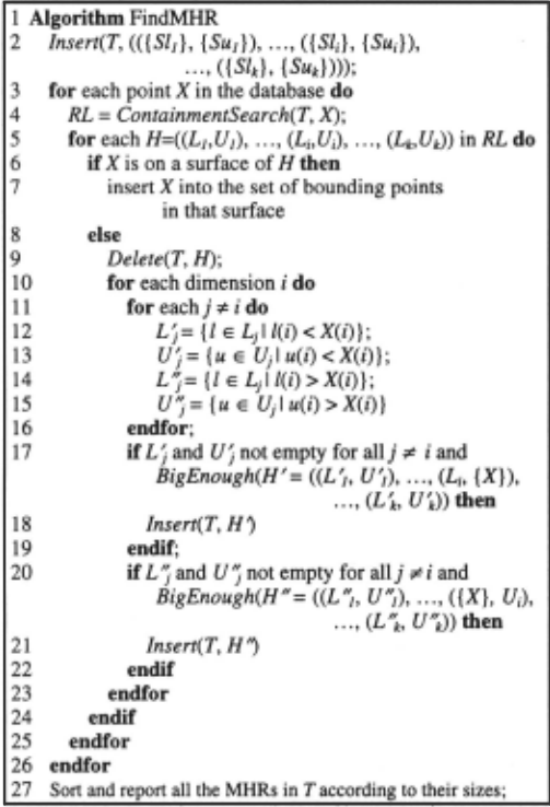
3.3 An example
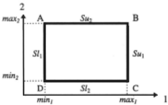
We use an example to illustrate the working of the algorithm. Suppose we have a 2-dimensional space S (ABCD) as shown in Figure 2. The first MHR is the whole space, ABCD, which is described with:
H = (({SlJ} , {Sui}), ({S/2}, {Su2})))
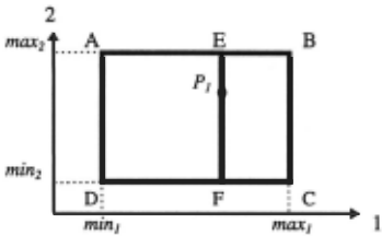
Line 3. We add the first point X= Pi to the inside of ABCD (see Figure 3).
Line 4. Since in this case there is only one MHR (the original space ABCD) contains Pi in T, thus
whereL1 = {SlJ}, Vi= {Sui}, L2= {S/2} and U2 ={Su2}.
RL = { ((Li, Ui), (L2, U2))}.
Line 5. The first MHR to be considered is
H = ((L~t Ui), (L2, U2)), i.e. ABCD in Figure 2 .
Line 6. Since P1 (Figure 3) is not on a surface of H, we pro ceed to Line 9.
Line 9. His deleted since it is no longer a MHR. It will be replaced with smaller MHRs.
Line 10. We split H along each dimension. Dimension 1 is considered first.
Line 11-16. In this part, we look for the sets of bounding points along dimension 2. L 2 and U 2 are the sets of lower and upper bounding points for the new MHR that will be formed to the left of Pi . L '2 and U '2 are the sets of lower and upper bounding points for the new MHR to be formed to the right side of P1. We obtain:
Line 17-19. It forms the new MHR H' that uses Pi as its up per bounding point on dimension 1, and L 2 and U 2 as its sets of lower and upper bounding points on dimen sion 2. Since in this case, both L 2 and U 2 are not empty, then
which is AEFD in Figure 3. Assume H'is big enough. It is inserted into T (Line 18).
Line 20-22. This forms the other new MHR H"that uses Pi as the lower bounding point on dimension 1. We obtain, H"= ({PJ}, {Sui}), ({S/2}. {Su2})),
which is EBCF in Figure 3. Assume H" is also big enough. It is inserted into T.
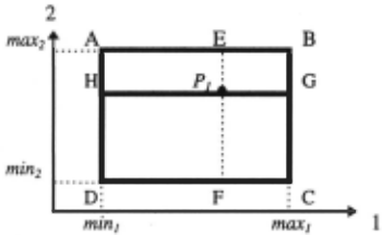
Line 10-16. Next, we consider dimension 2. We have:
L'i= {Sli}, U'i ={Sui}, and L'/= {Sli}, U'/ ={Sui}. Line 17-22. H'and H"are the two new MHRs formed due to P1 splitting the original MHR along dimension 2 (see Figure 4). We then have,
H'= (({SlJ}, {Sui}), ({S/2}, {Pi})) and
H"= (({SlJ}, {Su1 }), ({Pi}. {Su2})),
which are ABGH and HGCD in Figure 4 respectively.
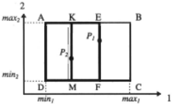
This ends adding the first point and updating T with the new MHRs. Let us now add another point, P2, into the space (see the location of P2 in Figure 5).
Line 4. The set of MHRs in T containing P2 is:
They are AEFD and HGCD respectively in Figure 4. Line 5-9. We consider the first MHR,
which is AEFD in Figure 5. Since P2 is not on a surface
H = (({Sl1}, {PJ}), ({Sl2}, {Su2})), of H, H is deleted.
Line 10. Assume dimension 1 is considered first.
Line 11-16. The bounding points obtained are:
L 2 = {Sl2}, U2 = {Su2}, and L '2 = {Sl2}, U'2 = {Su2} . Line 17-22. We obtain
H'= (({Sl1 }, {P2}), ({Sl2}, {Su2})) and
H"= (({P2}, {P1 }), ({Sl2}, {Su2})),
which are AKMD and KEFM respectively in Figure 5. Assume they are big enough. They are inserted into T,
Line 10-16. Consider dimension 2 w.r.t. the same MHR, H = (({Sl1 }, {PJ}), ({Sl2}, {Su2})). We obtain,
L'1= {Sl1}, U'1= {},andL'/= {Sl1}, U'/= {PJ}.
Note that in this case, U'1 = {} because the coordinate of P1 along dimension 1 is greater than the coordinate of P2 along dimension 1. See OF in Figure 6 (there is no point on OF). This means that there is no upper bounding point along dimension 1.
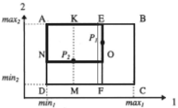
Line 17-22. There is no H 'because U'1 = { }. H'should be (if it exists) NOFD in Figure 6, but NOFD is not a MHR. Its space will be occupied later by another MHR. Here we only have H '~
H"= (({S/1}, {PJ}), ({P2}, {Su2})),
which is AEON in Figure 6.
Line 5. We now go back to work on the other MHR,
H = ( ( { Sl J}, { Su 1 }), ( { Sl2}, { P 1}))}, which is HGDC in Figure 4 or 7.
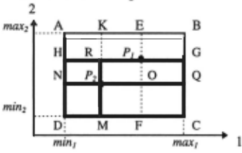
Line 6-21. After going though the similar process as the above, we obtain 3 new MHRs,
(( {P2}, {Su1 }), ( {Sl2}, {P1})) : RGCM in Figure 7,
(({Sl1}, {Su1 }), ({Sl2}, {P2})): NQCD in Figure 7,
(( {Sl1}, {Su1 }), ( {P2}, {P1 })) : HGQN in Figure 7.
Note that HRMD is not a MHR because there is no bounding point on HR, however, HRMD is inside the MHR AKMD formed earlier. NOFD, which was not in cluded in any new MHR when we consider AEFD, is now inside NQCD.
The final of sets of MHRs in T are RGCM, NQCD, HGQN, AKMD, KEFM, AEON, ABGH, EBCF respec tively in Figure 7.
3.4 Proof of correctness
A sketch of the proof of the correctness of the algorithm is presented next. We prove that the algorithm FindMHR pro duces all possible MHRs that have sizes accepted by the BigEnough() function. Hence, we need to show that any hy per-rectangle reported by FindMHR must be maximal and accepted by BigEnough(), and any given MHR that is ac cepted by BigEnough() in the space S must be reported. The former is easy to show as our algorithm checks each hyper rectangle before it is inserted into T. Hence we focus our attention on proving the latter.
The detailed proof is too long to be presented here, instead we give an outline of the proof (interested reader may refer to [Ku et al., 1997] for the detailed proof). Let us first as sume that BigEnough() accepts MHR of all sizes, i.e. , no pruning is done. Our task is to prove that the algorithm FindMHR finds all possible MHRs, i.e., the data structure T stores all possible MHRs. The proof will proceed in an in ductive manner, showing at the base case, when there is no point inserted, there is only 1 MHR which occupies the whole space. Then at each iteration, if T already stores all MHR before the next point X is inserted, by inserting X and performing all the necessary updates, T contains all resultant MHRs. This in turn is decomposed into several parts:
- Show that those MHRs in T not containing X will not be affected (which justifies the use of the function Contain mentSearch()).
- Show that those MHRs in T containing X will not be maximal anymore (which justifies why they are deleted).
- Show that the new MHRs must be inside the union of the MHRs found by ContainmentSearch() (which justifies why the new MHR are generated only from these MHR found).
- Show that the new MHRs must touch X and all possible MHRs that touch X will be reported (which justifies the way the new MHRs are constructed).
- Show that no identical MHRs can be generated using this algorithm (which justifies why we do not check for dupli cates).
A final point is that in our algorithm, the newly generated MHR is always contained within the MHR from which it is derived from, hence it is safe to discard any MHR that is not accepted by BigEnough() (by the definition of BigEnough()). With this, the correctness of the algorithm FindMHR is proved.
3.5 Run time complexity
Each insert and delete operation on T can be implemented in O((log mh amortized time, where there are O(m) number of MHRs stored in T. Containment search in T is done in O(log m + C) where there are 0( C) number of MHRs returned [Overmars and Leeuwen, 1982].
A loose bound on the total number of MHR (i.e., m) is O(n 2 <k-Il) since a possible MHR can be constructed by choosing 2(k-1) points from the n points, to bound the k-1 dimensions, and the bounding points for the last dimension is simply decided from the geometry. We also assume that the number of bounding points per MHR is small, thus the op eration to compute L j, U j, L '), L '}is almost constant.
With this assumption, the alforithm runs in O(n(log m + C) + nC(log m) 2 + nCk(Iog m) + nee) which simplifies to O(nCk(Iog m) 2 + nCk 2 ). Since Cis of O(m) and m is of O(n2k· 2 ), the run time is simplified to O(n2k-J ~(log n) 2 ).
Although this complexity is high, in practice the number of sufficiently large MHRs is not many. Thus, computational cost is usually not a problem.
4 Experimental Results
The proposed algorithm is implemented in C++. Two sets of experiments have been conducted to test the efficiency and effectiveness of the algorithm in discovering the MHRs. The first set of experiments aims to show that the running time of the algorithm is reasonable. All the datasets are randomly generated. Some areas are intentionally left empty. But we have no knowledge about the existence of holes in other ar eas. Here, we only present the results from the 3D datasets because they are more representative of the real-life situa tions. Holes of more than 3D are hard to understand (interested reader may refer to [Ku et al., 1997] for experi mental results using higher dimensional datasets). Let X, Y and Z denote the 3 dimensions. The resolution of X, Y and Z is of an accuracy of up to 1/100. We run the first set of experiments on 3 different datasets. The lower and upper bounds for X and Yin all the three datasets are 0.00-23 .00 and 0.00-17.00 respectively. The bounds for Z are 0.0020.00, 0.00-70.00 and 0.00-150.00 respectively for the three datasets. The planted empty areas are of the same size, 9, 6 and 9 along X, Y and Z dimensions respectively. Table 1 summarizes the run time results of the three datasets (running on Digital Alpha 8400 under normal loading conditions). Note that T (which stores all the MHRs) is currently imple mented as a linked list.
| Data set | No. of points | Running time a:b - a mins b sees | No. ofMHRs found | ||
|---|---|---|---|---|---|
| 8-4-8 | 4-2-4 | 8-4-8 | 4-2-4 | ||
| 1 | 1427 | 0:02 | 0:06 | 85 | 2299 |
| 2 | 5064 | 0: 15 | 1 : 05 | 162 | 6925 |
| 3 | 10702 | 1: 10 | 6: 17 | 260 | 13141 |
Column 1 indicates the dataset number. Column 2 shows the number of data points in each dataset. Column 3 gives the running times for finding all the MHRs that satisfy the mini mal length requirements along the 3 dimensions. This col umn is further divided into two sub-columns. One of them shows the running times when the minimal lengths along X, Y and Z dimensions of the MHRs are 8, 4 and 8 respectively (i.e., the bounds used by BigEnough()). The other shows the running times when the minimal length is reduced by half along each dimension (i.e., 4-2-4). Column 4 gives the num ber of MHRs discovered by the algorithm in each of the two situations. From the table, we see that when the minimal size of the MHR decreases, the time taken to find all the suffi ciently large MHRs increases. We also see that as the num ber of data points increases, the time taken to find all the large MHRs also increases. In general, however, the relation ship between the number of data points and the time taken to find all the large MHRs is complex because there are other factors that play a role, e.g., the density and/or the distribu tion of the data points, and the number of large MHRs that exist in the dataset. In all experiments, the running times are reasonable. In spite of the large number of discovered MHRs (both planted and unknown), many of them actually represent the same general regions with slight variations (slightly dif ferent sets of bounding points). In practice, post-processing can be performed to extract those general empty regions.
In the second set of experiments, we use a real-life disease dataset. This dataset has 7 continuous attributes, and 713 data points. The algorithm is run 8 times using different at tribute combinations, i.e., combining 2, or 3 or 4 attributes. The minimal size of the MHRs in each experiment is speci fied by a doctor. The running times of all the tests are within 1 or 2 seconds.
In these experiments, a number of interesting holes are discovered. For example, it is suspected that if the systolic blood pressure (SBP) of a subject is high, then his/her di systolic blood pressure (DBP) is also high. A hole is discov ered in the region of high SBP and low DBP. This hole con firms the suspected fact. Some holes are quite unexpected.
For instance, the doctor has a strong belief that the higher the SBP, the more likely the subject will get the disease. How ever, it is found that between the age of 18-50 (the upper bound of age is 69), there is no subject whose SBP is higher than 145 (the upper bound is 231) and is diagnosed to have the disease.
5 Related Work
To the best of our knowledge, no existing algorithm is able to find interesting holes in a multi-dimensional database. Although there are algorithms in geometry [Chazelle et al., 1986; Orlowski, 1990] that can find empty rectangles in the 2D space, these algorithms cannot be extended to the multi dimensional space.
Most current research in machine learning and machine discovery focuses on finding rules or formulae that exist in data. Our work is different from rule induction [e.g., Quinlan, 1992] because rule induction is not concerned with empty areas. It typically groups the empty areas with the data areas in order to arrive at some generalized rules.
Typical existing scientific discovery systems discover qualitative and numeric laws from data. Examples of well knoWn systems include ABACUS [Falkenhainer and Michal ski, 1986], BACON [Langley et al., 1987], FAHRENHEIT [Zytkow, 1990], and IDS [Nordhausen and Langley, 1993]. They are different from our work because our algorithm is targeted at discovering those empty areas, which may repre sent impossible value combinations.
Conceptual clustering systems [e.g., Fisher, 1987] typi cally partition the data cases into similar classes and form concept hierarchies. Again, they are not concerned with those empty areas that do not contain any data.
In data mining research, many techniques have been pro posed to discover regularities in data [Fayyad et al., 1996]. They are similar to those above for machine learning. Here, we would like to mention specifically the association rule discovery technique in [Agrawal et al., 1993]. This technique discovers associations that exist in the database whose attrib utes are all nominal (or discrete) attributes. For this type of databases, the concept of MHR does not apply. The equiva lent concept of MHR in the nominal case is missing associa tions. Since the algorithm in [Agrawal et al. , 1993] can find all the existing value associations in a database. Using a sim ple technique (e.g., generate and test), it is possible to find all the missing associations (without going through the database again). However, the problem is the efficiency and the repre sentation of the missing associations. In our future work, we will study this problem. This paper only focuses on discov ering those significant MHRs in a continuous space.
6 Conclusion
This paper argues that although discovering rules or regu larities that exist in data is important, in many situations, discovering of large holes in the database is also interesting. An algorithm that is able to discover holes in the continuous space, also known as maximal hyper-rectangles (MHR), is proposed and implemented. We believe this algorithm will be useful in scientific discovery and data mining.
Acknowledgments
We would like to thank Dr. Hing-Yan Lee, Ms. Hwee-Leng Ong and Ms. Angline Pang from Information Tehcnology Institute, and Dr. Ke-Qing Gong and Dr. King-Hee Ho from National University Hospital for many useful discussions, for providing us the databases, and for their help in the testing of our system.
@inproceedings{ijcai1997p134,
  title     = {Discovering Interesting Holes in Data},
  author    = {Liu, Bing and Ku, Liang-Ping and Hsu, Wynne},
  booktitle = {Proceedings of the Fifteenth International Joint Conference on
               Artificial Intelligence, {IJCAI-97}},
  publisher = {International Joint Conferences on Artificial Intelligence},
  editor    = {Martha E. Pollack},
  pages     = {930--934},
  year      = {1997},
  note      = {Learning},
  url       = {https://ijcai.org/proceedings/1997/134},
}
TY - CPAPER TI - Discovering Interesting Holes in Data AU - Liu, Bing AU - Ku, Liang-Ping AU - Hsu, Wynne T2 - Proceedings of the Fifteenth International Joint Conference on Artificial Intelligence, IJCAI-97 PB - International Joint Conferences on Artificial Intelligence PY - 1997 SP - 930 EP - 934 UR - https://ijcai.org/proceedings/1997/134 ER -Copied
Machine-readable versions of this paper, for tools and AI agents:





