
Learning Topological Maps with Weak Local Odometric Information
Proceedings of the Fifteenth International Joint Conference on Artificial Intelligence. Learning. Pages 920-928.
© 1997 International Joint Conferences on Artificial Intelligence
Abstract
Topological maps provide a useful abstraction for robotic navigation and planning. Although stochastic maps can theoretically be learned using the Baum- Welch algorithm, without strong prior constraint on the structure of the model it is slow to converge, requires a great deal of data, and is often stuck in local minima. In this paper, we consider a special case of hidden Markov models for robot-navigation environments, in which states are associated with points in a metric configuration space. We assume that the robot has some odometric ability to measure relative transformations between its configurations. Such odometry is typically not precise enough to suffice for building a global map, but it does give valuable local information about relations between adjacent states. We present an extension of the Baum- Welch algorithm that takes advantage of this local adometric information, yielding faster convergence to better solutions with less data.
- [Basye et al., 1995] K. Basye, T . Dean and L. P. Kaelbling. Learning dynamics: System identification for perceptually challenged agents. Artificial Intelligence, 72(1), 1995.
- [Cassandra et al., 1996] A. R. Cassandra, L. P. Kaelbling and J. A. Kurien. Acting under uncertainty: Discrete Bayesian models for mobile-robot navigation. In Proceed- ings of IEEE/RSJ International Conference on Intelligent Robots and Systems, 1996.
- [Cheeseman et al., 1990] P. Cheeseman et a/. Autoclass: A Bayesian classification system. In J. W. Shavlik and T. G. Dietterich, editors, Readings in Machine Learning, pages 296-306.
- [Dempster et al., 1977] A. P. Dempster, N. M. Laird and D. B. Rubin. Maximum likelihood from incomplete data via the EM algorithm . Journal of th e Royal Statistical Society, 39(1):1-38, 1977.
- [Engelson and McDermott, 1992] S. P. Engelson and D. V. McDermott. Error correction in mobile robot map learn- ing. In Proceedings of the IEEE International Confer- ence on Robotics and Automation, pages 2555-2560 , Nice , France, May 1992.
- [Juang et al., 1986] B. H. Juang, S. E . Levinson and M. M. Sondhi. Maximum likelihood estimation for multivariate mixture observations of Markov chains. IEEE Transac- tions on Information Theory, 32(2) , March 1986.
- [Juang, 1985] B. H. Juang. Maximum likelihood estimation for mixture multivariate stochastic observations of Markov chains. ATBT Technical Journal, 64(6), July-August 1985.
- [Koenig and Simmons, 1996a] S. Koenig and R. G. Sim- mons. Passive distance learning for robot navigation. In Proceedings of the Thirteenth International Conferen ce on Machine Learning, pages 266-274 , 1996.
- [I<oenig and Simmons, 1996b] S. Koenig and R. G. Sim- mons. Unsupervised learning of probabilistic models for robot navigation. In Proceedings of the IEEE International Conference on Robotics and Automation, 1996.
- [Kuipers and Byun, 1991] B. Kuipers and Y.-T. Byun. A robot exploration and mapping strategy based on a seman- tic hierarchy of spatial representations. Journal of Robotics and Autonomous Systems, 8:47-63, 1991. .
- [Kullback and Leibler, 1951] S. Kullback and R. A. Leibler. On information and sufficiency. Annals of Mathemati cal Statistics, 22(1) :79-86, 1951.
- [Liporace, 1982] L. A. Liporace. Maximum likelihood esti- mation for multivariate observations of Markov sources. IEEE Transactions on Information Theory, 28(5) , 1982 .
- [Nourbakhsh et a/., 1995] I.
- Nourbakhsh , R. Powers and S. Birchfield. Dervish: An office-navigating robot. A I Magazine, 16(1):53-60, 1995 .
- [Pierce and Kuipers, 1997] D. Pierce and B. Kuipers. Map learning with uninterpreted sensors and effectors. Artificial Intelligence, 1997. (To appear) .
- [Rabiner, 1989] L. R. Rabiner. A tutorial on hidden Markov models and selected applications in speech recognition. Proceedings of the IEEE, 77(2):257-285, February 1989.
- [Shatkay and Kaelbling, 1997] H. Shatkay and L. P. Kael- bling. Learning hidden Markov models with geometric information. Technical Report CS-97-04, Department of Computer Science, Brown University, April 1997.
- [Simmons and Koenig, 1995] R. G. Simmons and S. Koenig. Probabilistic navigation in partially observable environ- ments. In Proceedings of the International Joint Confer- ence on Artificial Intelligence, 1995.
- [Thrun and Biicken, 1996a] S. Thrun and A. Biicken. Inte- grating grid-based and topological maps for mobile robot navigation. In Proceedings of the Thirteenth National Con- ference on Artificial Intelligence, pages 944-950, 1996.
- [Thrun and Biicken, 1996b] S. Thrun and A. Biicken. Learn- ing maps for indoor mobile robot navigation. Techni- cal Report CMU-CS-96-121, School of Computer Science, Carnegie Mellon University, Pittsburgh, PA , April 1996.
References were extracted automatically from the PDF and may contain errors.
Full text extracted automatically from the PDF; figures, tables and equations may differ. The PDF is the version of record.
1 Introduction
Hidden Markov models (HMMs), as well as their exten sion to partially observable Markov decision processes (POMDPs) model a variety of nondeterministic ~ynami cal systems as abstract probabilistic state-transitwn sys tems with discrete states, observations and possibly ac tions. 1 Such models have proven particularly useful as a basis for robot navigation in buildings, providing a sound method for localization and planning [Simmons and Koenig, 1995; Nourbakhsh et al., 1995; Cassandra et al., 1996]. Much previous work has required that the model be specified manually; this is a tedious process and it is often difficult to obtain correct probabilities.
An ultimate goal is for an agent to be able to learn such models automatically, both for robustness and in order to cope with new and changing environments. The Baum-Welch algorithm [Rabiner, 1989] is frequently used to learn HMMs. Since POMDPs are a simple exten sion of HMMs, they can, theoretically, be learned with a simple extension to the Baum-Welch algorithm. How ever, without strong prior constraint on the structure of the model, the Baum-Welch algorithm does not perform very well: it is slow to converge, requires a great deal of data, and is often stuck in local minima.
1 Actions are modeled by POMDPs but not by HMMs.
In this paper, we consider a special case of HMMs (extendable to POMDPs) for robot navigati?n, in which states are associated with points in a metnc configura tion space. We assume the robot has some odometric ability to measure relative transformations between its configurations. Such odometry is typically not ?recise enough to suffice for building a global map, but It does give valuable local information about relations between adjacent states. This information is readily available in most robots and is often ignored during the process of learning topological maps. We present an extension ~f the Baum-Welch algorithm that takes advantage of this local odometric information, yielding faster convergence to better solutions with less data.
2 Related Work
There has been a great deal of work on learning maps for mobile robotics and on learning stochastic models of dynamical systems in general. In this section, we focus on map learning for robots.
Sometimes it is necessary for a robot to know its lo cation accurately in terms of metric coordinates; in such cases, metric maps are clearly the best choice. In many other environments, such as office buildings with cor ridors and rooms, or networks of roads, maps that sim ply specify the topology of important locations and their connections suffice. Such maps are typically less complex and support much more efficient planning than metric maps. Topological maps are built on lower-level abstrac tions that allow the robot to move along arcs (perhaps by wall- or road-following) and to recognize properties of the locations; they are flexible in allowing a more gen eral notion of state, possibly including information such as the robot's battery voltage or whether or not it is holding a bagel.
There are two typical strategies for deriving topolog ical maps: one is to learn the topological map directly; the other is to first learn a geometric map, then to derive a topological map through some process of analysis.
A nice example of the second approach is provided by Thrun and Biicken [1996b; 1996a], who use occupancy grid techniques to build the initial map. This strategy is appropriate when the primary cues for decomposition and abstraction of the map are geometric. However, in many cases, the nodes of a topological map are defined in terms of other sensory data (e.g. labels on a door). Learning a geometric map first also relies on the ado metric abilities of a robot; if they are weak and the space large, it is very difficult to derive a consistent map.
We take the approach of learning the topological map directly, assuming that abstraction of the robot's per ception and action abilities has already been done (we do it by hand, but see work of Pierce and Kuipers [1997] for an automatic method). Some approaches learn an underlying deterministic map of the world, independent of the noise in the robot's sensing and action processes. We prefer to learn a combined model of the world and the robot's interaction with the world; this allows ro bust planning that takes into account likelihood of error in sensing and action.
Kuipers and Byun [1991] provide a strategy for learn ing deterministic topological maps. It works well in do mains in which most of the noise in the robot's percep tion and action is abstracted away, learning from single visits to nodes and traversals of arcs. It is unable to han dle situations in which long strings of actions and obser vations are necessary to disarpbiguate the robot's loca tion. Another set of learning algorithms, based on the theory of learning deterministic finite state automata, work in much noisier environments with much less global information. Basye, Dean, and Kaelbling [1995] provide algorithms for learning deterministic maps given fairly strong assumptions; these algorithms come with proba bilistic correctness guarantees for learning in polynomial time with a polynomial amount of data.
Engelson and McDermott [1992]learn "diktiometric" maps (topological maps with metric relations between nodes) from experience. The uncertainty model they use is interval based rather than probabilistic, and the learned representation is deterministic. Ad hoc routines handle problems resulting from failures of the uncer tainty representation.
The work most closely related to ours is by Koenig and Simmons [l996b; 1996a], who learn POMDP models (stochastic topological maps) of a robot hallway environment. They also recognize the impossibility of learning such a model without initial information; they solve the problem by using a human-provided topological map, to gether with further constraints on the shared structure of the model. A modified version of the Baum-Welch al gorithm learns the parameters of the model. They also developed an incremental version of Baum-Welch that allows it to be used on-line in certain kinds of environ ments. Their models contain very weak metric informa tion, representing hallways as chains of one-meter seg ments and allowing the learning algorithm to select the most probable chain length. This method is effective, but results in large models with size proportional to the hallways length.
We show that, by using odometric information di rectly, we can avoid the use of a priori models and still learn stochastic maps efficiently and effectively.
3 Models and Assumptions
In the following sections, we describe the model and algo rithms used for learning an HMM, rather than a POMDP. Extension to POMDPs is technically straightforward but notationally more cumbersome.
The world is composed of a finite set of states. The states do not necessarily correspond directly to locations of the robot; they may include other state information, such as orientation or battery level. The dynamics of the world are described by state-transition distributions that specify the probability of making transitions from one state to the next. There is a finite set of observations that can be made in each state; the frequency of such ob servations is described by a probability distribution and depends only on the current state. In our model, ob servations are multi-dimensional, so an observation is a vector of values, each chosen from a finite domain. It is assumed that observation values are conditionally inde pendent, given the state. Each state is assumed to be associated with a point in some metric space. Whenever a state transition is made, the robot records an odometry vector, which estimates the location of the current state relative to the previous state. It is assumed that the components of the odometry vector are corrupted with independent normal noise (extension to dependent noise is possible, and requires reestimation of the complete co variance matrix).
More formally, a model ts a tuple .>. (S, 0, A, B, R, 1r), where
- S = { St, ... , SN} is a finite set of N states;
- 0 = TI~=l 0; is a finite set of observation vectors of length l; the ith element of an observation vector is chosen from the finite set 0;;
- A is a stochastic transition matrix, with A;,j = Pr(qt+t = sjiQt = s;); 1"'S_i,j"'S_N; Qt is the state at
timet;
- B is an array of l stochastic observation matri ces, with B;,j,o = Pr(vt[i] = o!qt = sj); 1 ~ i ~ l, 1 ~ j ~ N, o E Oj; Vt is the observation vector at timet;
- R is a relation matrix, specifying for each pair of states, s; and Sj, the mean and variance of the D-dimensional metric relation between them; J.L(R;,j[k]) is the mean of the kth component of the relation between s; and Sj and o- 2 (R;,j[k]), the variance; furthermore, R is geometrically consistent: for each component k, the relation Rk(a, b) ~r J.L(Ra,b[k]) must be a directed metric, sat isfying the following properties for all states a, b, and c:
- o Rk(a,a) = 0;
- o Rk(a, c)= Rk(a, b)+ Rk(b, c) (additivity);
- 1r is a stochastic initial probability vector describing the distribution of the initial state; for simplicity it is assumed here to be (1, 0, 0, ... , 0}, implying that the robot is always started in state s0 .
A learning algorithm starts from an initial model >.; and is given a sequence of experience E; it returns a revised model >., with the goal of maximizing Pr(E!>.). The experience sequence E is of length T; each element is a pair (rt, vt}, where rt is the observed relation between qt-1 and qt and vt is the observation vector at time t .
To extend the above model to a POMDP, actions need to be introduced into the model. Each possible action is associated with a separate set of three matrices A, B and R. In addition, each item in the experience sequence E contains the action which caused the transition and the observation associated with it. The algorithmic com plexity oflearning a POMDP compared with that oflearn ing an HMM is within a factor proportional to the number of possible actions, which is usually much smaller than the number of states.
4 Algorithm
Our algorithm is a straightforward extension of Baum Welch to deal with the relational information and the factored observation sets. The Baum-Welch algorithm is an expectation-maximization (EM) algorithm [Dempster et al., 1977]; it alternates between
- the E-step of computing the state-occupation prob abilities 1 at each time in the sequence given E and the current model >., and
- the M-step of finding a new model ). that maximizes Pr(E!>., I)·
An EM algorithm is guaranteed to provide monotoni cally increasing convergence of Pr(E!>.). Baum-Welch has been proven to be an EM algorithm; it has also been provably extended to real-valued observations [Liporace, 1982; Juang, 1985]. Our algorithm introduces an addi tional matrix, and enforces the first two geometric con sistency constraints on the M-step, but like the standard Baum-Welch it is still guaranteed to converge to a local maximum of the likelihood function [Shatkay and Kael bling, 1997]. The proof is along the lines of the one presented by Juang et al [1986] for the standard Baum Welch algorithm, and is beyond the scope of this paper.
4.1 Computing State-Occupation Probabilities
Following Rabiner [1989], we first compute the forward (a) and backward (,13) matrices. When all measurements are discrete, at(i) is the probability of observing Eo through Et and qt = s;, given >.; and f3t ( i) is the proba bility of observing Et+l through ET-l given qt = s; and >.. When some of the measurements are continuous (as is the case with R), these matrices contain probability density values rather than probabilities.
The forward procedure for calculating the a matrix is initialized with
and continued for 0 < t ~ T - 1 with
where f(rt!R;,j) is the density at point rt according to the normal distribution represented by the means and variances in entry i, j of the relation matrix R, and b{ is the probability of observing vector Vt in state Sj; that is, . I fT: = ili=l B;,j,v,[iJ ·
The backward procedure for calculating the j3 matrix is initialized with
and continued for 0 ~ t < T - 1 with
Given a and /3, we now compute the state-occupation and state-transition probabilities (I and~ respectively). The state-occupation probabilities are computed as fol lows:
Similarly, the state-transition probabilities are computed as:
We note that the numerator and the denominator in the fractions are both density functions, but the quotient is a discrete probability function. These are essentially the same formulae appearing in [Rabiner, 1989), but taking into account the density of the relational observation.
4.2 Updating Model Parameters
In this phase of the algorithm, the goal is to find a new model, A, that maximizes P(EIA, 1). Generally, this is done by simple maximum-likelihood estimation of the probability distributions in A and B by computing ex pected transition and observation frequencies. It is more difficult in our model, because we must also compute a new relation matrix, R, under the constraint that it re main geometrically consistent.
The A and B matrices can be straightforwardly re estimated; A;,j is the expected number of transitions from s; to Sj divided by the expected number of transi tions from s;:
and B;,j,o is the expected number of times o is observed along the ith dimension when in Sj divided by the ex pected number of times of being in Sj:
where J(c) is an indicator function with value 1 if c is true and 0 otherwise.
If we were not going to enforce geometrical consis tency, then the R matrix would be re-estimated by:
In the current implementation, we enforce only two of the three constraints of geometrical consistency. Zero distances between states and themselves are trivially en forced. Anti-symmetry is enforced by using the data from Sj to s; as well as from s; to Sj when reestimat ing J..L(R;,j)· Thus the actual reestimation formula for J..L(R;,j) is:
The additivity constraint is not currently enforced through the updates, although it is satisfied in the ini tial models, thus biasing the learned model towards sat isfying it. We are exploring some relaxation techniques, based on spring systems, for enforcing the additivity con straint. The complexity of the algorithm per iteration is still O(TN 2 ), like the standard Baum-Welch.
4.3 Finding an Initial Model
It is typical in instances of the Baum-Welch algorithm to simply initialize the model at random, perhaps try ing multiple initial models to find different local like lihood maxima. We have tried random initial models, as well as starting from a more informed model, based on the odometry information. In both the random and informed initializations the initial R matrix satisfies all three properties of geometrical consistency.
To build an informed model, we begin by assigning global metric coordinates to each element in the sequence E. This is done by accumulating the observed relations between consecutive pairs of states. This data set (ig noring other observation information) is fed into a simple k-means clustering algorithm, yielding a clustering of the data into N clusters. The clusters are taken to be the states, and the observations associated with a given clus ter are interpreted as having been generated in the asso ciated state. We then compute 1 and~ values, with the 1 values being 0 or 1, since we use a deterministic cluster ing algorithm (it might be beneficial to use a stochastic clustering algorithm, such as Autoclass [Cheeseman et al., 1990)). The A, B, and R matrices are all estimated from 1 and ~ as described in the previous section. Fi nally, an ad hoc process is used to adjust R to satisfy the additivity constraint.
5 Experiments
The goal of this work is to use odometry to improve the learning of topological models, while using fewer it erations and less data. We tested our algorithm in a simple robot-navigation world. Our experiments consist of running the algorithm both on data obtained from a simulated model and on data gathered by our mobile robot, Ramona, which is a modified RWI B21 robot. It has a cylindrical synchro-drive base, 24 ultrasonic sen sors and 24 infrared sensors, situated evenly around its circumference. The infrared sensors are used mostly for short-range obstacle avoidance. The ultrasonic sensors are longer ranged, and are used for obtaining (noisy) observations of the environment. The amount of data gathered by Ramona is used here as a proof of concept but is not sufficient for statistical analysis. For the lat ter, we use data obtained from the simulated model.
5.1 Robot Domain
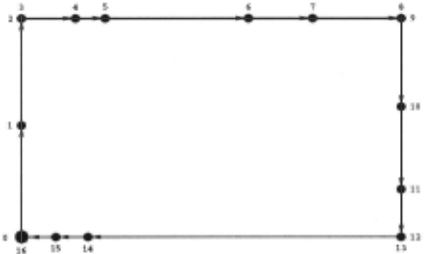
The robot follows a prescribed path through the cor ridors in an office environment. Low-level software pro vides a level of abstraction that allows the robot to move through hallways from intersection to intersection and to turn ninety degrees to the left or right. At each intersec tion, ultrasonic data interpretation allows the robot to perceive, in each of the four cardinal directions, whether there is an open space, a door, a wall, or something un known. The robot also identifies doors and openings that it passes along the corridors. Of course, both the action and perception routines are subject to error. Fi nally, the robot has encoders on its wheels that allow it to estimate its pose (position and orientation) with re spect to its pose at the previous intersection. The path Ramona followed consists of 4 connected corridors in our building, which include 17 states, as shown in Figure 1.
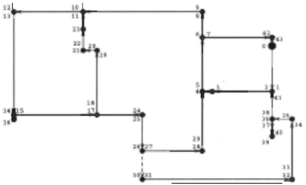
In our simulation, we manually generated an HMM representing a prescribed path of the robot through the complete office environment, consisting of 44 states, and the associated transition, observation, and odometric distributions. Figure 2 shows the HMM corresponding to the simulated hallway environment 2 . Further interpre tation of the figures is provided in the following section.
5.2 Evaluation Method
There are a number of different ways of evaluating the re sults of a model-learning algorithm. None is completely satisfactory, but they all give some insight into the utility of the results.
In this domain, there are transitions and observations that usually take place, and are therefore more likely than the others. Furthermore, the relational information gives us a rough estimate of the metric locations of the states. To get a qualitative sense of the plausibility of a learned model, we can extract an essential map from the learned model, consisting of the states, the likely tran sitions and the metric measures associated with them ' and ask whether this map corresponds to the essential map underlying the true world.
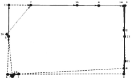
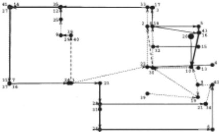
Figures 1 and 2 are such essential versions of the true maps, while Figures 3 and 4 are essential versions of rep resentative learned maps. Black dots represent the phys ical locations of states. Multiple states (depicted as num bers in the plot) associated with a single location typi cally correspond to different orientations of the robot at that location. The larger black circle represents the ini tial state. Arrows represent transitions that have prob ability 0.2 or higher. Solid arrows represent the most likely transitions between the states, and dashed arrows represent the less likely ones 3 · Note that the length of the arrows is significant and represents the length of the corridors, drawn to scale.
2 Observations and orientation are omitted for clarity.
More traditionally, in simulation experiments, the learned model is quantitatively compared to the actual model that generated the data. Each of the models in duces a probability distribution on strings of observa tions; the asymmetric Kullback-Leibler divergence [Kull back and Leibler, 1951] between the two distributions is a measure of how good the learned model is with respect to the true model. Given a true probability distribution P ::::: {Pl, ... , Pn} and a learned one Q = { q1, ... , qn}, the KL divergence of Q with respect to P is:
We report our results in terms of a sampled version of the KL divergence, as described by Rabiner [1989]. It is based on generating sequences of sufficient length (5 sequences of 1000 observations in our case) according to the distribution induced by the true model, and compar ing their likelihoods according to the learned model with the true model likelihoods. We ignore the odometry in formation when applying the KL measure, thus allowing comparison between models that are learned with and without odometry.
5.3 Results
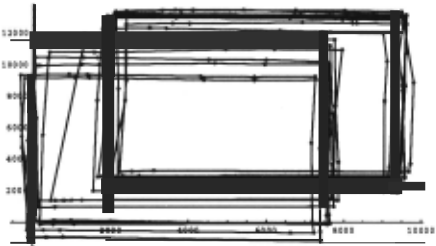
We let Ramona go around the path depicted in Fig ure 1 and collect a sequence of about 300 observations. Figure 5 plots the sequence of metric coordinates ob tained by accumulating consecutive odometric readings (as described in Section 4.3). We applied the learning algorithm to the data 40 times. 20 of these runs were started from an informed (cluster based) initial model and 20 started from a random initial model. (Note that there is non-determinism even when using informed ini tial models, since the clustering starts with random k means, t_hus multiple runs give multiple results).
3 Bold dashed arrows represent transitions that are almost as likely as the most likely.
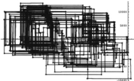
Figure 3 shows an essential representation of a typical learned map starting from an informed model. The ge ometry of the learned map strongly corresponds to that of the true map, and most of the states positions were learned correctly. Although the figure does not show it, the learned observation distributions at each state match well with the true observation distributions. When start ing from an uninformed model, the results were not as satisfactory, which was predictable.
For obtaining statistically sufficient information, we generated 5 data sequences, each of length 1000, using Monte Carlo sampling from the model shown in Figure 2. One of these sequences is depicted in Figure 6. The figure demonstrates that the noise model used in the simulation is indeed compatible with the noise pattern associated with real robot data.
We used three different settings of the learning algo rithm:
- starting from an informed (cluster based) initial model and using odometry information;
- starting from a random initial model and using odometry information;
- starting from a random initial model without using odometry information (standard Baum-Welch).
For each sequence and each of the three algorithmic set tings we ran the algorithm repeatedly 5 times. In all the experiments, N was set to be 44, which is the "correct" number of states; for generalization, it will be necessary to use cross-validation or regularization methods to se lect model complexity.
Figure 4 shows the essential version of one learned map (obtained from the sequence of Figure 6) for a rep resentative run. We note that some of the states whose locations overlap in the true model (e.g. 8,9) become sep arated in the learned model (e.g. 33,17,3), due to noise in the odometry readings and observations. However, there is an obvious correspondence between groups of states in the learned and true models, and most of the transitions (as well as the observations, which are not shown) were learned correctly.
| Seq. | Informed I | Random I | No Odo I | |||
|---|---|---|---|---|---|---|
| # | KL | Iter. # | KL | Iter. # | KL | Iter. # |
| I | 2.347 | 93.40 | 3.797 | IIO.OO | 10.129 | 201.80 |
| 2 | 2.338 | 84.00 | 2.630 | 82.00 | 11.400 | 213.80 |
| 3 | 2.572 | 85.80 | 3.086 | 150.00 | l1.583 | 195.40 |
| 4 | 3.185 | 85.20 | 3.532 | l14.20 | 11.810 | 224.00 |
| 5 | 4.154 | 116.20 | 3.877 | 102.40 | 12.258 | 156.80 |
Table 1 lists the KL divergence between the true and learned model, as well as the number of runs until conver gence was reached, for each of the 5 sequences under each of the 3 learning settings, averaged over 5 runs per se quence. From the table it is clear that the KL divergence with respect to the true model for models learned using odometry, starting from either an informed or a random initial model, is about 4 times smaller than for models learned without odometry data. The standard deviation around the means was about 1.5 for all KL distances. To check the significance of our results we used the simple two-sample t-test. The models learned using odometric information have statistically significantly (p < 0.005) lower average KL divergence than the others.
In addition, the number of iterations required for con vergence when learning using odometry information is roughly half that required when ignoring odometry in formation. Again, the t-test verifies the significance of this result.
The initial clustering strongly biases the outcome of learning; it is important to understand whether this bias is useful. When the entire model is initialized at random, the convergence time (measured in number of iterations) as well as the KL measure are somewhat higher on aver age, than when starting at an initial model based on clus tering. The difference between the two starting points is not highly statistically significant since the clustering in many cases is not good. When the initial clustering is good, most of the work is already done and the EM algorithm quickly fills in the details. However, if the initial clustering is bad, it is often close to a poor local minimum and the algorithm is unable to adjust it well. It will be important to try more sophisticated clustering algorithms. It may be best to run the algorithm mul tiple times, some with initial clustering and some with out, taking the model with the highest likelihood as the final result.
To examine the influence of the amount of data on the quality of the learned models, we took one of the 5 sequences (Seq. #1) and used its prefixes of length 100 to 1000 (the complete sequence), in increments of 100, as individual sequences. We ran each of the three algorithmic settings over each of the 10 prefix sequences, 10 times repeatedly. We then used the KL-divergence as described above to evaluate each of the resulting models with respect to the true model. For each prefix length we averaged the KL-divergence over the 10 runs.
| Seq. | Informed | Random | No Odo | |||
|---|---|---|---|---|---|---|
| length | Mean KL | Std. Dev. | Mean KL | Std. Dev. | Mean KL | Std. Dev. |
| 1000 | 2.097 | 0.71 | 3.016 | 1.24 | 10.139 | 1.90 |
| 800 | 1.805 | 0.28 | 2.954 | 1.75 | 13.319 | 1.26 |
| 600 | 2.353 | 1.14 | 2.569 | 1.36 | 14.542 | 1.62 |
| 400 | 2.953 | 0.60 | 2.801 | 1.69 | ' 22 .714 | 4.69 |
| 300 | 3.998 | 1.53 | 3.892 | 3.50 | -+ 00 | NA |
| 200 | 9.169 | 3.09 | 7.489 | 5.25 | -+ 00 | NA |
| 100 | -+ 00 | NA | -+ 00 | NA | -+ 00 | NA |
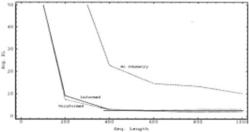
Table 2 summarizes the results of this experiment. It lists the mean KL-divergence over the 10 runs for each of the prefixes, as well as the standard deviation around this mean. Entries with KL-divergence -t oo indicate that sequences generated by the true model were as signed negligible (-o) probability by the learned model, which corresponds to an infinite KL-divergence. The plot in Figure 7 depicts the KL-divergence as a function of the sequence length for each of the three settings. Both the table and the plot demonstrate that, in terms of the KL-divergence, our algorithm, which uses odometric in formation, is robust in the face of data reduction. In contrast, learning without the use of odometry is much more sensitive to reduction in the amount of data.
Again, we applied the two-sample t-test to verify the statistical significance of these results. For example, the KL-divergence being greater for sequences of length 800 than for sequences of length 1000 when learning with out the use of odometry is highly statistically significant (p « 0.005). In contrast, the KL-divergence is not statis tically significantly greater when the odometry is used, for either informed or uninformed models. The informed model is even somewhat better, (with moderate statis tical significance, p < 0.11), when using the sequence of length 800, due to better clustering when there is less accumulated noise on the odometry data.
We note that the data sequence is twice as "wide" when odometry is used than when it is not, that is, there is more information in each element of the sequence when odometry data is recorded. However, the effort of record ing this additional odometric information is negligible, and is well rewarded by the fact that fewer observations and Jess exploration are required for obtaining a data sequence sufficient for adequate learning.
6 Conclusions
Odometric information, which is often readily available, makes it possible to learn HMMs (or POMDP models) for robot navigation efficiently and effectively. If we are interested in learning the geometric relationships be tween states, using the odometry readings is obviously very helpful. Moreover, our experiments show that even when we are only interested in the underlying topologi cal model, using odometry can both reduce the number of iterations required by the algorithm and improve the resulting model, while requiring shorter data sequences.
The work described in this paper is fairly preliminary. In the very near future, we will extend the example to learn the fully controllable POMDP rather than the HMM. The current implementation uses a very naive clustering algorithm; it will be useful to investigate more sophis ticated clustering methods. The algorithm described in this paper is a batch algorithm. It would be useful to adapt it to be an incremental on-line algorithm. Finally, we would like to find an improved M-step that would preserve the additivity constraint.
Acknowledgments
We thank Jim K uri en for providing and supporting the low level code for Ramona, and William Smart and Ja son Lango for helping to keep her alive. We are also indebted to John Hughes for the term "additivity" and Sam Trychin for letting us use his skateboard.
This work was supported in part by the Air Force and ARPA under grant No. F30602-95-l-0020, by the NSF in conjunction with ARPA under grant No. IRI-9312395, and by the NSF under grant No. IRI-9453383.
@inproceedings{ijcai1997p133,
  title     = {Learning Topological Maps with Weak Local Odometric Information},
  author    = {Shatkay, Hagit and Kaelbling, Leslie Pack},
  booktitle = {Proceedings of the Fifteenth International Joint Conference on
               Artificial Intelligence, {IJCAI-97}},
  publisher = {International Joint Conferences on Artificial Intelligence},
  editor    = {Martha E. Pollack},
  pages     = {920--928},
  year      = {1997},
  note      = {Learning},
  url       = {https://ijcai.org/proceedings/1997/133},
}
TY - CPAPER TI - Learning Topological Maps with Weak Local Odometric Information AU - Shatkay, Hagit AU - Kaelbling, Leslie Pack T2 - Proceedings of the Fifteenth International Joint Conference on Artificial Intelligence, IJCAI-97 PB - International Joint Conferences on Artificial Intelligence PY - 1997 SP - 920 EP - 928 UR - https://ijcai.org/proceedings/1997/133 ER -Copied
Machine-readable versions of this paper, for tools and AI agents:





