
Look-Ahead Value Ordering for Constraint Satisfaction Problems
Proceedings of the Fourteenth International Joint Conference on Artificial Intelligence. Constraint Satisfaction. Pages 572-577.
© 1995 International Joint Conferences on Artificial Intelligence
Abstract
Looking ahead during search is often useful when solving constraint satisfaction problems. Previous studies have shown that looking ahead helps by causing dead-ends to occur earlier in the search, and by providing information that is useful for dynamic variable ordering. In this paper, we show that another benefit of lo?king ahead is a useful domain value ordermg heuristic, which we call look-ahead value ordering or LVO. LVO counts the number of times each value of the current variable conflicts with some value of a future variable, and the value with the lowest number of conflicts is chosen first. Our experiments show that look-ahead value ordering can be of substantial benefit, especially on hard constraint satisfaction problems.
- Peter Cheeseman, Bob Kanefsky, and William M. Taylor. Where the really hard problems are. In &78 CONSTRAINT SATISFACTION Proceedings of the International Joint Conference on Artificial Intelligence, pages 331-337, 1991. IJCAI
- Rina Dechter. Enhancement Schemes for Constraint Processing: Backjumping, Learning, and Cutset Decomposition. Artificial Intelligence , 41 :273-312, 1990.
- Rina Dechter and Judea Pearl. Network-based heuristics for constraint-satisfaction problems. Ar- tificial Intelligence, 34:1-38, 1987.
- Daniel Frost and Rina Dechter. In search of the best constraint satisfaction search. In Proceedings of the Twelfth National Conference on Artificial In- telligence, pages 301-306, 1994.
- J . Gaschnig. Performance measurement and anal- ysis of certain search algorithms. Technical Report CMU-CS-79-124, Carnegie Mellon University, 1979.
- R. M. Haralick and G. L. Elliott. Increasing Tree Search Efficiency for Constraint Satisfaction Prob- lems. Artificial Intelligence, 14:263-313, 1980. IJCAI
- David Mitchell, Bart Selman, and Hector Levesque. Hard and Easy Distributions of SAT Problems. In Proceedings of the Tenth National Conference on Artificial Intelligence, pages 459-465, 1992.
- Judea Pearl. Heuristics. Addison-Wesley, Reading, Mass., 1985.
- Patrick Prosser. Hybrid Algorithms for the Con- straint Satisfaction Problem. Computational Intel- ligence, 9{3):268-299, 1993.
- Paul Walton Purdom. Search Rearrangement Back- tracking and Polynomial Average Time. Artificial Intelligence, 21 :117-133, 1983.
- Norman Sadeh and Mark S. Fox. Variable and Value Ordering Heuristics for Activity-based Job- shop Scheduling. In Proceedings of the Fourth Inter- national Conference on Expert Systems in Produc- tion and Operations Management, pages 134-144, 1990.
- Ramin Zabih and David McAllester. A Rearrange- ment Search Strategy for Determining Propositional Satisfiability. In Proceedings of the Seventh Na- tional Conference on Artificial Intelligence , pages 155-160, 1988.
References were extracted automatically from the PDF and may contain errors.
Full text extracted automatically from the PDF; figures, tables and equations may differ. The PDF is the version of record.
1 Introduction
In this paper we present a new heuristic for prioritizing the selection of values when searching for the solution of a constraint satisfaction problem. Because the task of finding a solution for a constraint satisfaction problem is NP-complete, it is unlikely that any solution technique exists that works well in all cases. Nevertheless, many al gorithms and heuristics have been developed which p.ro vide substantial improvement over simple backtrackmg (depth-first search) on many problem in~tances. I! a con straint satisfaction problem has a solutiOn, knowmg the right value for each variable would enable a solution to be found in a backtrack-free manner.
When a constraint satisfaction problem has only a small number of solutions, much time is often spent searching branches of the search space which do not lead to a solution. To minimize backtracking, we should first try the values which are more likely to lead to a consis tent solution. Even a slight increase in the probability that a value chosen is part of a solution can have sub stantial impact on the time required to find a solution.
*This work was partially supported by NSF grant IRI9157636, by the Electrical Power Research Institute (EPRI), and by grants from Toshiba of America, Xerox Northrop and Rockwell.
Our new algorithm, look-ahead value ordering {LVO), implements a heuristic that ranks the values of a vari able based on information gathered by looking ahead, determining the compatibility of each value with the val ues of all future variables. Although the heuristic does not always accurately predict which values will lead to solutions, it is frequently more accurate than an unin formed ordering of values. Our experiments show that while the overhead of LVO usually outweighs its ben efits on easy problems, the improvement on very large problems can be substantial. Interestingly, LVO often improves the performance of backjumping on problems without solutions, as well.
Look-ahead value ordering does the same type oflook ahead as does the forward checking algorithm [6]. Be cause forward checking rejects values that it determines will not lead to a solution, it can be viewed as doing a simple form of value ordering. In this regard LVO is more refined, because it also orders the values that may be part of a solution.
In the following section we define formally constraint satisfaction problems and describe the look-ahead value ordering algorithm. Section 3 describes the experiments we conducted. In section 4 we discuss the results of these experiments. We review some related approaches in section 5 and in section 6 summarize our results.
2 Definitions and Algorithms
A constraint satisfaction problem {CSP) is represented by a constraint network, consisting of a set of n variables, X1, .. . ,Xn; their respective value domains, D1, .. . ,Dn; and a set of constraints. A constraint is a subset of the Cartesian product Di 1 x ... x Di;, consisting of all tu ples of values for a subset (X it> .·. , Xi;) of the ~ari~bles which are compatible with each other. A solutwn IS an assignment of values to all the variables such that no con straint is violated; a problem with a solution is termed satisfiable or consistent. Sometimes it is desired to find all solutions; in this paper, however, we focus on the task of finding one solution, or proving that no solution ex ists. A binary CSP is one in which each of the constraints involves at most two variables. A constraint satisfaction problem can be represented by a constraint graph which has a node for each variable and an arc connecting each pair of variables that are contained in a constraint.
2.1 Algorithms and Heuristics
We experimented with look-ahead value ordering by test ing it in conjunction with an algorithm that combines backjumping, dynamic variable ordering, and the tem porary pruning of future domains characteristic of for ward checking. Previous experiments have shown that this combination is extremely effective over a wide range of problems [4]. LVO (or any other heuristic) is of prac tical interest only if it improves upon the performance of state of the art algorithms.
Backjumping
Backjumping [5; 2] is an improvement to backtracking which takes advantage of sparseness and structure in the constraint graph. Both backtracking and backjumping consider each variable in order, instantiating the current variable, X cur, with a value from its domain Dcur that does not violate any constraint between Xcur and all previously instantiated variables. If Xcur has no such non-conflicting value, then a dead-end occurs. The ver sion of backjumping we use, based on Prosser's conflict directed backjumping [9], is very effective in choosing the best variable to jump back to.
There are two basic ways to determine which values in D; are consistent with all variables before X;. Look back methods consider each element in D; and check to ensure that no constraints with earlier variables are vio lated. There are also several look-ahead approaches, the simplest being forward checking [6]. When assigning a value to the current variable, forward checking removes values from the domains of future variables that con flict with that value. We will refer to the subset of D; that has incompatible values removed as Di. When X; is reached, the only values remaining in Di are those which are consistent with all previous variables, as in stantiated. If a value x E Di had been removed because it conflicted with the instantiation of an earlier variable Xh, then X has to be restored when Xh is assigned a new value, or is jumped over in backjumping.
Dynamic variable ordering ·
In a dynamic variable ordering (DVO) scheme [6; 10; 12] the order of variables can be different in different branches of the search tree. Our implementation of DVO uses information derived from a forward checking style look-ahead. At each step the variable with the smallest remaining domain size is selected. If Di is empty for some uninstantiated variable X;, then X; is moved to be the next variable, and a dead-end occurs immediately. The technique for breaking ties is important, as there are often many variables with the same domain size. In our implementation we maintain a list of the variables sorted by degree in the original constraint graph, and in case of a tie (and for the first variable), choose the one highest on this list. This scheme gives substantially bet ter performance than picking one of the tying variables at random.
Look-ahead value ordering
Backjumping and dynamic variable ordering can be com bined into an algorithm we call BJ+DVO [4]. The BJ+DVO algorithm does not specify how to choose a
Backjumping with DVO and LVO
Inputs: A set of n variables, X1, ... , Xn;
For each X;, a set D; of possible values (the domain) .
Uses: For each X;, a mutable domain set Di of values not proven inconsistent with the current partial assignment (initially, all D' =D);
For each X;, a set P; of earlier variables which, as instantiated, conflict with some value in D; (initially, all P = 0).
Output: All variables instantiated, or failure.
- If the current variable is the last variable, then all variables have value assignments; exit with this solution. Otherwise,
- (a) (Dynamic variable ordering.) Select the uninstantiated variable X; with the small est remaining domain Di and make it the next variable in the ordering; call it X cur. Set Pcur = 0.
- (b) (Look-ahead value ordering.) Rank the val ues in D~ur: For each value x in D~ur, ex amine each uninstantiated variable X;. For each X;, examine each v in Di. Compute (using one ofthe heuristics described in Sec tion 3.2) the rank of x based on whether X; = v conflicts with Xcur = x, and on the resulting size of Di .
- Select a value x E D~ur . Do this as follows:
- (a) If D~ur = 0, go to 3.
- (b) Choose the highest ranked value x in D~ur, and remove it from D~ur· (Without LVO, choose x arbitrarily.)
- (c) (With LVO this step can be avoided by caching the results from 1(b).) Examine each uninstantiated variable X;. For each X;, examine each v in Di. If X; = v con flicts with Xcur = x, then remove v from Di and add X cur toP;. If a Di becomes empty, then go immediately to (d).
- (d) Instantiate X cur = x and go to 1.
- (Backjump.) If Pcur = 0 (there is no previ ous variable), exit with failure. Otherwise, let Xjump = the latest variable in Pcur, and remove Xjump from Pcur· Let Pjump = Pjurrp U Pcur· For all i, jump < i ~ cur, set P; = W and set Di = D;. Set Xcur = Xjump· Go to 2.
Figure 1: Backjumping with dynamic variable ordering and look-ahead value ordering (BJ+DVO+LVO). Re moving step 1(b) leaves plain BJ+DVO.
| Parameters N, K, T, C | No LVO | LVO-MC | LVO-MD | LVO-WMD | LVO-PDS |
|---|---|---|---|---|---|
| 25, , 1 , 9 | 54,44 | , 1 | 47,7 | 5,19 | , 1 |
| 250, 3, 3/9, 391 | 75,174 | 58,253 | 62,343 | 67,742 | 58,253 |
| 35, 6, 4/36, 501 | 603,271 | 562,440 | 597,234 | 608,364 | 571,471 |
| 50, 6, 8/36, 325 | 397,242 | 372,309 | 387,475 | 386,132 | 372,747 |
| 35, 9, 27/81, 178 | 249,099 | 230,030 | 237,134 | 237,690 | 238,710 |
| 100, 12, 110/144, 120 | 1,786,829 | 332,895 | 822,649 | 915,982 | 403,781 |
| 50, 20, 300/400, 95 | 1,400,338 | 942,079 | 1,034,031 | 1,081,250 | 979,723 |
value. In our experiments reported in [4], and in this paper when we refer to "plain" BJ+DVO, values are ar bitrarily assigned a sequence number, and are selected according to this sequence. In this paper we explore the feasibility of using information gleaned during the look-ahead phase of BJ+DVO to improve the ordering of values. The method we use to rank the values in or der of decreasing likelihood of leading to a solution is as follows. The current variable is tentatively instantiated with each value in its domain D'. With each value in D', LVO looks ahead to determine the impact this value will have on the D' domains of uninstantiated variables. We discuss in section 3.2 four heuristic functions that use information from the look-ahead to rank the values in the current domain. The current variable is then instan tiated with the highest ranking value. If the algorithm backjumps to a variable, the highest ranked remaining value in its domain is selected. If the variable is re instantiated after earlier variables have changed, then the order of the values has to be recalculated. The LVO heuristic will not always make the right decision. How ever, a small improvement in an algorithm's ability to choose the right value can have a big impact on the work required to solve a problem.
A high-level description of BJ+DVO+LVO is given in Fig. 1. To avoid repeating consistency checks, our im plementation saves in tables the results of looking ahead in step 1(b ). After a value is chosen, the D's and Ps of future variables are copied from these tables instead of being recomputed in step 2(c). BJ+DVO uses O(n 2 k) space for the D' sets, where k is the size of the largest domain: n levels in the search tree (D' is saved at each level so that it does not have to be recomputed after backjumping) x n future variables x k values for each future variable. Our implementation of BJ+DVO+LVO uses O(n 2 k 2 ) space. There is an additional factor of k because at each level in the search tree up to k values are explored by look-ahead value ordering. Similarly, the space complexity for the P sets increases from O(n 2 ) in BJ+DVO to O(n 2 k) for BJ+DVO+LVO. To solve a typical problem instance described in the next sec tion, BJ+DVO required 1,800 kilobytes of random access memory, and BJ+DVO+LVO required 2,600 kilobytes. On most computers the additional space requirements of LVO will not be severe.
3 Experimental Methods and Results
3.1 Instance Generator
The experiments reported in this paper were run on ran dom instances generated using a model that takes four parameters: N, K, T and C. The problem instances are binary CSPs with N variables, each having a domain of size K. The parameter T (tightness) specifies a fraction of the K 2 value pairs in each constraint that are disal lowed by the constraint. The value pairs to be disallowed by the constraint are selected randomly from a uniform distribution, but each constraint has the same fraction T of such incompatible pairs. T ranges from 0 to 1, with a low value ofT, such as 1/9, termed a loose or re laxed constraint. The parameter C specifies the number of constraints out of the N * (N - 1)/2 possible. The specific constraints are chosen randomly from a uniform distribution.
Certain combinations of parameters generate prob lems of which about 50% are satisfiable; such problems are on average much more difficult than those which all have solutions (under-constrained) or which never have solutions (over-constrained) [1; 7]. Such a set of param eters is sometimes called a cross-over point. For a given value of N, KandT, we call the value of C which pro duces 50% solvable problems "Ceo».
3.2 LVO Heuristics
The BJ+DVO+LVO algorithm in Fig. 1 does not spec ify exactly how information about conflicts with future variables should be used to prioritize the values of the current variable. We experimented with four heuristics that rank values by looking ahead.
The first heuristic, called min-conflicts (MC), consid ers each value in D' of the current variable and associates with it the number of values in the D' domains of future variables with which it is not compatible. The current variable's values are then selected in increasing order of this count.
The other three heuristics are inspired by the intuition that a subproblem is more likely to have a solution if it doesn't have variables with only one value. The max domain-size (MD) heuristic therefore prefers the value that creates the largest minimum domain size in the fu ture variables. For example, if after instantiating Xcur with value X1 the miJlte{cur+l, ... ,nJ I D; I is 2, and with Xcur = x2 the min is 1, then x1 will be preferred.
| ConsiStency ~ec!s | CPU seconds | |||||||||||
|---|---|---|---|---|---|---|---|---|---|---|---|---|
| Parameters | Mean JL | Medtan | J1 | Hest | Mean | 11 -~est | ||||||
| N,K,T,C | uvu | LVU | Ralio | Jl DVO | LVO | Ralio | Jl_!{._atlo | ~ | ~ | Ralio | Jl Ratio | |
| Solvable and unsolval e mstances: | ||||||||||||
| 125, 3, 1(9, 929 | 254 ( 7~) | 226 ( 8%) | 0.89 | 214 | 187 | 0.87 | 4.81 | 10.1 | 10.5 | 1.04 | 0.47 | |
| 350, 3, 3/9, 524 | 2,365 {98%) | 1,130 {131%) | 0.48 | 7 | 5 | 0.69 | 1.26 | 1096.1 | 503.5 | 0.46 | 1.26 | |
| 350, 3, 1/9, 2292 | 3,251 {33%) | 509 {42%) | 0.16 | 350 | 18 | 0.05 | 3.59 | 331.2 | 62.1 | 0.19 | 3.20 | |
| 100, 12, 110/144, 120 | 1,787 (108%) | 333 {68%) | 0.19 | 24 | 20 | 0.83 | 1.55 | 189.1 | 37.8 | 0.20 | 1.14 | |
| 50, 20, 300/400, 95 | 1,400 {30%) | 942 {19%) | 0.67 | 368 | 293 | 0.79 | 3.48 | 53.6 | 39.1 | 0.73 | 0.91 | |
| Unsolvable mstances only: ll J I II | ||||||||||||
| 125, 3, 1(9, 929 | 354 ( 7%) | I 344 ( 7%) | I 0.97 | 316 | 304 | I 0.96 II | 14.94ll | 14.0 | 16.0 | 1.14 | 0.00 | |
| 350, 3, 3/9, 524 | 4,028 {119~) | 2,354 {1U%) | 0.58 | 32 | 23 | 0.74 | 2.51 | 1953.1 | 1054.2 | 0.54 | 1.90 | |
| 350, 3, 1/9, 2292 | 1 All instances had solutions - C is 90% of the crossover point ~ | |||||||||||
| 100, 12, 110/144, 120 | 3,048 {156~) | I 548 {105%) | I 0.18. | 44l | 35 I | 0.80 If | 3.58] | 316.1 | I 62.0 | I 0.20 | II 1.42 | |
| 50, 20, 300/400, 95 | 1,052 (24%) | 923 (24%) | 0.88 | 316 | 291 | 0.92 | 5.31 | 39.6 | 37.7 | 0.95 | 0.65 | |
| Solvable mstances only: | ||||||||||||
| 125, 3, ~(9, 929 | 150 (12%) | 102 (16%) | 0.68 | 118 | 51 | 0.44 | 2.50 | 6.1 | 4.9 | 0.81 | 1.88 | |
| 350, 3, 3/9, 524 | 1,027 {160%) | 145 (122%) | 0.14 | 4 | 4 | 0.95 | 0.80 | 406.2 | 60.1 | 0.15 | 0.92 | |
| 350, 3, 1/9, 2292 | 3,251 (33%) | 509 {42%) | 0.16 | 350 | 18 | 0.05 | 3.59 | 331.2 | 62.1 | 0.19 | 3.20 | |
| 100, 12, 110/144, 120 | 1,059 {123%) | 209 {62%) | 0.20 | 18 | 14 | 0.78 | 1.03 | 115.7 | 23.9 | 0.21 | 1.00 | |
| 50, 20, 300/400, 95 | 2,047 (55%) | 977 {30%) | 0.48 | 446 | 318 | 0.71 | 1.92 | 79.5 | 41.7 | 0.52 | 1.71 | |
Since several values in the domain of the current vari able D~ur may create future D's of the same size, the MD heuristic frequently leads to ties. A refined version of MD is weighted-max-domain-size (WMD). Like MD, WMD prefers values that leave larger future domains, but it break ties based on the number of future vari ables that have a given future domain size. Continuing the example from the previous paragraph, if x1 leaves 3 variables with domain size 2 (and the rest with do main sizes larger than 2), and X3 leaves 5 variables with domain size 2, then x1 will be preferred over x3 .
Our fourth heuristic, called point-domain-size (PDS), gives each value in D~ur a point value: 8 points for each future domain of size 1; 4 points for each future domain of size 2; 2 points for each future domain of size 3 (if I< > 3); and 1 point for each future domain of size 4 (if I< > 4). The value with the smallest sum of points is chosen first.
Fig. 2 shows the results of experiments comparing the four LVO heuristics. In terms of mean consistency checks, LVO usually improves BJ+DVO no matter which heuristic is chosen. Since the MC heuristic was clearly best, we selected it for further experimentation. In the rest of the paper, reference to LVO implies the MC heuristic.
3.3 Experimental results
The overall conclusion we draw from our experiments comparing BJ+DVO with BJ+DVO+LVO is that on sufficiently difficult problems LVO almost always produces substantial improvement; on medium problems LVO usually helps but frequently hurts; and on easy problems the overhead of LVO is almost always worse than the benefit. Very roughly, "sufficiently difficult" is over 1,000,000 consistency checks and "easy" is under 10,000 consistency checks.
We experimented further with LVO by selecting sev eral sets of parameters and with each set generating 500 instances that were solved with both BJ+DVO and BJ+DVO+LVO. We used two approaches for select ing combinations of parameters which had large values of N and K, and yet did not generate problems that were too computationally expensive. The first strategy was to use very tight constraints and very sparse con straint graphs. For instance, problems at N=100 and K=12 would be extremely time consuming to solve, ex cept that we used a small number (C=120) of extremely tight constraints (T=ll0/144). Another method for gen erating easier problems with large N and K is to select parameters that are not exactly at the cross-over point. We used this approach for the experiment with N=350, K=3, T=1/9 and C=2292, which is 90% of the estimated ceo of 2547.
The results of these experiments are summarized in Fig. 3. We present the data in several ways: the ta ble show the mean, the median, and the ratio of how many times each algorithm was better than the other. The "Ratio" columns under "Mean" and "Median" in Fig. 3 provide an indication of the relative performance of the two algorithms. Mean ratios and median ra.tios less than one indicate that BJ+DVO+LVO is bet ter than BJ+DVO (required fewer consistency checks or CPU time). In the "Best Ratio" column a larger num ber indicates superior performance by BJ+DVO+LVO, as this figure is the number of times BJ+DVO+LVO was better then BJ+DVO, divided by the number of times BJ+DVO bested BJ+DVO+LVO (as measured by con sistency checks or CPU time) .
For many uses, the mean is the most relevant statis tic, as it takes into account the impact of the occasional extremely difficult problem. To convey an estimate of the accuracy of our sample of 500 instances, we provide, for the consistency check measure, the size of the 95% confidence interval, expressed as a percentage of the sam ple mean. The 95% confidence interval around the true population mean JJ is computed as
where i is the sample mean, u is the population standard deviation, tis the number of trials, and 1.96 is the factor associated with the 95% confidence interval. Since we don't actually know the standard deviation of the entire population, we have to estimate it by using the sample standard deviation; this is acceptable as long as t > 30, but still introduces another source of possible inaccuracy.
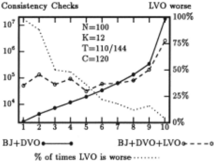
The medians in Fig. 3 are much lower than the means, because in each sample there were a small number of ex tremely difficult problems, and a few very difficult ones. In our experiments with N=100, K=12, T=ll0/144 and C= 120 half the CPU time was spent solving the hardest 25 of the 500 problems. Fig. 4 shows the skew in the distribution, and how LVO affects problems of different difficulties. For this figure, the 500 instances in one ex periment were divided into ten groups of 50, based on the number of consistency checks required by BJ+DVO.
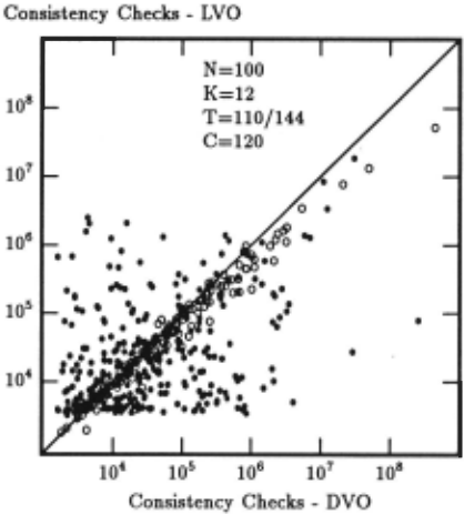
The easiest 50 were put in the first group, the next easi est 50 in the second group, and so on. LVO is harmful for the first several groups, and then produces increasingly larger benefits as the problems become more difficult . The scatter chart in Fig. 5 also indicates the distribu tion of the data. (Due to space constraints, some of our figures show data drawn from only one parameters, such as N=100, K=12, T=ll0/144, C=120. The charts of data from experiments with other parameters are quite similar.)
In general the statistics for CPU time are slightly less favorable for LVO than are the statistics for Consistency Checks, reflecting the fact that, in our implementation, there is approximately a 5%-10% performance penalty in CPU time for LVO. This is caused by the need to store and copy the large tables that hold the results of look ing ahead on different values of a variable (the caching referred to in Step 2( c) of Fig. 1). Many problem in stances required slightly fewer consistency checks with LVO but slightly more CPU time, resulting in the often substantially different "Consistency Checks Best Ratio" and "CPU seconds Best Ratio" numbers in Fig. 3.
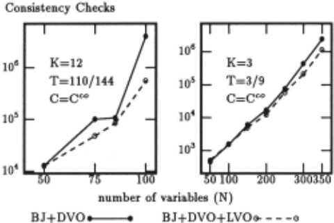
The graphs in Fig. 6 show that the impact of LVO increases as the number of variables increase. Moreover, when variables have small domain sizes, a larger number of variables is required for LVO to have a beneficial im pact. For instance, at N=75 and K=12, LVO improves BJ + DVO substantially, while with the small domain size K=3, the impact ofLVO does not appear until N is larger than 200.
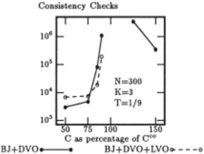
The efficacy of LVO also depends on how near the pa rameters are to the 50% solvable crossover point. As the data in Fig. 7 indicate, LVO is detrimental on very easy underconstrained problems (with C less than around 80% of ceo) that have many solutions. On these prob lems, the extra work LVO does exploring all values of a variable is almost always unnecessary. When problems are sufficiently overconstrained ( C greater than around 125% of ceo), LVO has very little effect on the number of consistency checks.
In addition to experimenting with LVO on random problems, we compared BJ+DVO and BJ+DVO+LVO on several scheduling problems that had been trans formed into graph coloring problems. In each case the impact of LVO was minimal, except for a slight degra dation in CPU time. The symmetrical nature of graph coloring constraints does not provide any information that look-ahead value ordering can exploit.
4 Discussion
With backtracking the order in which values are chosen makes no difference on problems which have no solu tion, or when searching for all solutions. Therefore it may be surprising that a value ordering scheme can help BJ+DVO on instances that are unsatisfiable, as the data in Fig. 3 and Fig. 5 indicate. As the following theorem states, the reason is the interaction between backjump ing and look-ahead value ordering.
Theorem 1 When searching for all solutions, or on problems which have no solution,
- the order in which values are chosen does not affect the search space which backtracking explores; and
- the order in which values are chosen can affect the search space which backjumping explores.
Proof. Part 1: Consider a search tree rooted at variable X. The n children of X are X 1 , X 2, ... , Xn . The size of the search space SS(X) of this tree is 1 + 2:~=1 SS(X;). Since addition is commutative and the search spaces of the children do not interact, the or der in which the search spaces rooted at the children of X are expanded will not affect SS(X).
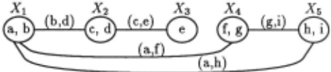
Part 2: Consider the problem depicted in Fig. 8, and assume X1 = a is assigned first. There are two value orders for X2. If X2 = cis considered first, then X3 will be a dead-end. x2 = d will be instantiated next, and an eventual dead-end at X5 will lead to a jump back to X4 and then to X1 . (X2 and X3 will be jumped over because they are not connected to X4 or X5. ) On the other hand, if x2 = d is considered first, a different search space is explored because X2 = c is never encountered. Instead, X2 and Xa are jumped over after the dead-ends at X4 and Xs. 0
Note that the theorem holds whether a look-ahead or look-back method is used, and whether the variable or dering is static or dynamic. LVO can help on unsatisfi able problems, and on unsatisfiable branches of problems with solutions, by more quickly finding a consistent in stantiation of a small set of variables which are later jumped over by backjumping.
5 Related Work
Value ordering techniques have been investigated be fore, but they have not been based on information de rived from a forward checking style look-ahead. Pearl [8] discusses similar value ordering heuristics in the con text of the 8-Queens problem. His "highest number of unattacked cells" is the same as our max-conflicts heuris tic, and his "row with the least number of unattacked cells" heuristic is the same as max-domain-size.
Dechter and Pearl [3] developed an Advised Backtrack algorithm which estimates the number of solutions in the subproblem created by instantiating each value. The es timate is based on a tree-like relaxation of the remainder of the problem. For each value, the number of solutions is counted, and the count is used to rank the values. Advised Backtrack was the first implementation of the general idea that heuristics can be generated from a re laxed version of the problem instance.
Sadeh and Fox [11] also use a tree-like relaxation ofthe remaining problem, in the context of job-shop scheduling problems. Their value ordering heuristic considers as well the impact of capacity constraints and demand on scarce resources.
6 Conclusions and Future Work
We have introduced look-ahead value ordering, an al gorithm for ordering the values in a constraint satisfac tion problem. Our experiments show that for large and hard problems, LVO can improve the already very good BJ+DVO·algorithm by over a factor of five.
One drawback of LVO is that it is somewhat com plex to implement, as it uses a set of tables to cache the results of values that have been examined (during the ranking process) but not yet instantiated. Manipulat ing these tables incurs a small CPU overhead. Another disadvantage of LVO is that on easy solvable problems, where there are many solutions and hence many accept able value choices, it is usually detrimental. LVO need lessly examines every value of each variable along the almost backtrack-free search for a solution.
LVO is almost always beneficial on difficult instances that require over 1,000,000 consistency checks. Unex pectedly, it even helps on problems without solutions when used in conjunction with backjumping. We have tested LVO using a forward checking level of look-ahead. We plan to explore the possibility that a more compu tationally expensive scheme, such as partial look-ahead or full look-ahead [6] or directional arc consistency [3], will pay off in the increased accuracy of the value order ing. Another research direction is to reduce the over head of LVO on easy problems. This might be achieved by only employing value ordering in the earlier levels of the search, or by having value ordering automatically "turn off'' when it notices that current values are in con flict with relatively few future values, indicating an un derconstrained problem. A simple way to eliminate the overhead of LVO on very easy problems would be to al ways run a non-LVO algorithm first; if that algorithm has not completed by, say, 100,000 consistency checks, it is cancelled and problem solving is restarted with an LVO version. At the price of 100,000 extra consistency checks on some difficult problems, the costs of LVO on the easy majority of problems is avoided.
@inproceedings{ijcai1995p75,
  title     = {Look-Ahead Value Ordering for Constraint Satisfaction Problems},
  author    = {Frost, Daniel and Dechter, Rina},
  booktitle = {Proceedings of the Fourteenth International Joint Conference on
               Artificial Intelligence, {IJCAI-95}},
  publisher = {International Joint Conferences on Artificial Intelligence},
  editor    = {Chris S. Mellish},
  pages     = {572--577},
  year      = {1995},
  note      = {Constraint Satisfaction},
  url       = {https://ijcai.org/proceedings/1995/75},
}
TY - CPAPER TI - Look-Ahead Value Ordering for Constraint Satisfaction Problems AU - Frost, Daniel AU - Dechter, Rina T2 - Proceedings of the Fourteenth International Joint Conference on Artificial Intelligence, IJCAI-95 PB - International Joint Conferences on Artificial Intelligence PY - 1995 SP - 572 EP - 577 UR - https://ijcai.org/proceedings/1995/75 ER -Copied
Machine-readable versions of this paper, for tools and AI agents:





