
Combining the Predictions of Multiple Classifiers: Using Competitive Learning to Initialize Neural Networks
Proceedings of the Fourteenth International Joint Conference on Artificial Intelligence. Connectionist Models. Pages 524-530.
© 1995 International Joint Conferences on Artificial Intelligence
Abstract
The primary goal of inductive learning is to generalize well - that is, induce a function that accurately produces the correct output for future inputs. Hansen and Salamon showed that ,_ u~der certain assumptions, combining the predrctwns of several separately trained neural networks will improve generalization . One of their key assumptions is that the individual networks should be independent in the errors they produce. In the standard way of perform_ing backpropagation this assumption may be vrolated, because the standard procedure is to _initialize network weights in the region of werght space near the origin. This means that backpropagation's gradient-descent search may only reach a small subset of the possible local minima . In this paper we present an approach to initializing neural networks that uses competitive learning to intelligently create networks that are originally located far from the origin of weight space, thereby potentially increasing the set of reachable local minima. We report experiments on two real-world datasets where combinations of networks initialized with our method generalize better than combinations of networks initialized the traditional way.
- [Baxt, 1992] W. Baxt. Improving the accuracy of an artificial neural network using multiple differently trained networks. Neural Camp., 4:772-780, 1992.
- [Berenji and Khedkar, 1992] H. Berenji and P. Khedkar . Learning and tuning fuzzy logic controllers through re- inforcements. IEEE Transactions on N eural Networks , 3:724-740 , 1992 .
- [Drucker et al., 1994] H. Drucker, C. Cortes, L. Jackel, Y. Le Cun, and V. Vapnik . Boosting and other machine learning algorithms. In Procs . of the 11th Int. Machine Learning Con[, pages 53-61, New Brunswick , NJ , 1994.
- [Fahlman and Lebiere, 1990] S. Fahlman and C. Lebiere. The cascade-correlation learning archi- tecture . In D. Touretzky, editor, Advances in Neural Information Processing Systems , volume 2, pages 524- 532 .
- Morgan Kaufmann, 1990 .
- [Fahlman, 1988] S. Fahlman. Faster learning variations on back-propagation: An empirical study. In Procs. of the 1988 Connectionist Models Summer School, pages 38-51, Pittsburgh, PA, 1988.
- [Ghosh et al. , 1992] J. Ghosh, L. Deuser, and S. Beck. Evidence combination techniques for robust classifi- cation of short-duration oceanic signals. In SP IE Con[ on Adaptive and Learning Systems, volume 1706, pages 266-276, Orlando , FL , 1992 .
- [Granger, 1989] C. Granger. Combining forecasts - twenty years later. J. of Forecasting, 8 , 1989 .
- [Hampshire and Waibel, 1990] J. Hampshire and A. Waibel. A novel objective function for im- proved phoneme recognition using time-delay neural networks. IEEE Trans. on Neural Networks , 1:216- 228 , 1990.
- [Hansen and Salamon , 1990] L. Hansen and P. Salamon. Neural network ensembles. IEEE Trans. on Pattern Analysis and Machine Intelligence , 12:993-1001, 1990.
- [Hashem et al., 1993] S. Hashem, Y. Yih, and B. Schmeiser. An efficient model for product alloca- tion using optimal combinations of neural networks . In C. Dagli , L. Burke , B. Fernandez, and J. Ghosh , editors , Intelligent Engineering Systems through Arti- ficial Neural Networks, volume 3. ASME Press, 1993 .
- [Hecht-Nielsen , 1988] R . Hecht-Nielsen. Applications of counterpropagation networks. Neural Networks , 1:131-139, 1988.
- [Hinton, 1989] G. Hinton. Connectionist learning proce- dures . Artificial Intelligence, 40 :185-234, 1989.
- [Huang and Lippmann, 1988] W . Huang and R. Lipp- mann . Neural net and traditional classifiers . In D. Touretzky, editor , Advances in Neural Information Processing Systems , volume 1, pages 387-396.
- Morgan Kaufmann, 1988 .
- [Jacobs et al., 1991] R. Jacobs, M. Jordan, S. Nowlan, and G. Hinton. Adaptive mixtures of local experts. Neural Computation, 3:79-87 , 1991.
- [Kearns and Seung, 1995] M. Kearns and H. Seung. Learning from a population of hypotheses. Machine Learning, 18:255-276, 1995.
- [Lang et al., 1990] K. Lang, A. Waibel, and G . Hinton . A time-delay neural network architecture for isolated word recognition. Neural Networks, 3:23-43, 1990.
- [Le Cun et al., 1989] Y. Le Cun , J. Denker , and S. Solla. Optimal brain damage. In D. Touretzky, editor, Ad- vances in Neural Information Processing Systems , vol- ume 2, pages 598-605.
- Morgan Kaufmann, 1989.
- [Leng et al., 1994] B. Leng, B. Buchanan, and H . Nicholas. Protein secondary structure prediction using two-level case-based reasoning. In J. of Compu- tational Biology, pages 25-38 , 1994.
- [Lincoln and Skrzypek, 1990] W . Lincoln and J. Skrzy- pek . Synergy of clustering multiple back propagation networks. In D. Touretzky, editor, Advances in Neu- ral Information Processing Systems, volume 2, pages 650-659.
- Morgan Kaufmann, 1990.
- [Maclin and Shavlik, 1993] R. Maclin and J. Shavlik. Using knowledge-based neural networks to improve algorithms: Refining the Chou-Fasman algorithm for protein folding. Machine Learning, 11:195-215, 1993.
- [Mani, 1991] G . Mani. Lowering variance of decisions by using artificial neural network portfolios. Neural Computation, 3:484-486 , 1991.
- [Moody and Darken, 1988] J . Moody and C. Darken . Learning with localized receptive fields . In Proceed- ings of the 1988 Connectionist Models Summer School, pages 133-143, Pittsburgh , PA, 1988.
- [Moody and Darken , 1989] J. Moody and C . Darken. Fast learning in networks of locally-tuned processing units. Neural Computation, 1:281-294 , 1989.
- [Nguyen and Widrow , 1990] D . Nguyen and B . Widrow. Improving the learning speed of 2-layer neural net- works by choosing initial values of the adaptive weights . In Procs. IJCNN-90, volume 3, pages 21-26, San Diego, CA, 1990.
- [Opitz and Shavlik, 1993] D. Opitz and J . Shavlik. Heuristically expanding knowledge-based neural net- works . In Procs. IJCAI-93, pages 1360-1365 , Cham- bery, France , 1993 . IJCAI
- [Perrone and Cooper , 1994] M. Perrone and L. Cooper. When networks disagree: Ensemble method for neural networks. In R. Mammone, editor , Artificial Neural Networks for Speech and Vision. Chapman and Hall, 1994.
- [Perrone, 1992] M. Perrone. A soft-competitive split- ting rule for adaptive tree-structured neural networks. In Procs. IJCNN-92, pages 689-693 , Baltimore, MD, 1992.
- [Qian and Sejnowski, 1988] N. Qian and T. Sejnowski. Predicting the secondary structure of globular pro- teins using neural network models. J. of Molecular Biology, 202:865-884, 1988.
- [Quinlan, 1987] J. R. Quinlan. Simplifying decision trees. Int. Journal of Man-Machine Studies, 27:221- 234, 1987.
- [Reilly et al., 1987] R . Reilly, C. Scofield, C. Elbaum, and L. Cooper . Learning system architectures com- posed of multiple learning modules . In Procs. ICNN- 87, pages 495-503 , San Diego, CA , 1987.
- [Rogova, 1994] G . Rogova. Combining the results of several neural-network classifiers. Neural N etworks, 7:777-781 , 1994.
- [Rost and Sander, 1993] B. Rost and C. Sander . Predic- tion of protein secondary structure at better than 70% accuracy. J. of Molecular Biology, 232 :584-599, 1993.
- [Rumelhart and Zipser, 1985] D. Rumelhart and D. Zipser. Feature discovery by competitive learning. Cognitive Science , 9:75-112 , 1985 .
- [Rumelhart et al., 1986] D. Rumelhart, G . Hinton, and R . Williams. Learning internal representations by er- ror propagation. In D. Rumelhart and J . McClel- land, editors, Parallel Distributed Processing, Volume 1, pages 318-363 . MIT Press, 1986.
- [Schapire, 1990] R. Schapire . The strength of weak learnability. Machine Learning, 5:197-227, 1990.
- [Shen, 1992] W .-M . Shen . Complementary discrimina- tion learning with decision lists . In Procs. AAAI-92, pages 153-158, San Jose, CA, 1992 .
- [Wolpert, 1992] D. Wolpert . Stacked generalization. Neural Networks, 5:241-259 , 1992.
- [Zhang et al., 1992] X. Zhang, J. Mesirov , and D. Waltz. Hybrid system for protein secondary structure predic- tion. J. of Molecular Biology, 225 :1049-1063, 1992.
References were extracted automatically from the PDF and may contain errors.
Full text extracted automatically from the PDF; figures, tables and equations may differ. The PDF is the version of record.
1 Introduction
The main goal of classification learning is generaliza tion .- being able to induce a concept that accurately ~lassrfies future examples. The difficulty with achiev mg good generalization is that a learner cannot mea sure generalization directly; instead, the learner relies on its inductive bias to hopefully produce an accurate classifier. A number of schemes have been introduced to a~dre~s this_ ~biquitous problem, ran&ing from tree prunmg m decrswn trees [Quinlan, 1987j to the use of co~plexity terms in neural networks [Hinton, 1989]. In t~rs paper we present a way to address the generaliza tion _problem for neural networks trained by backprop agatron [Rumelhart et al., 1986]. Our solution employs Jude W. Shavlik Computer Sciences Department University of Wisconsin 1210 West Dayton Street Madison, WI 53706 USA
*This research was partially supported by ONR Grant
N00014-93-l-0998 and NSF Grant IRI-9002413.
the previously explored approach [Drucker et al., 1994; Hansen and Salamon, 1990; Lincoln and Skrzypek 1990· Rogova, 1994] of training a set of networks rathe~ thru: a single network and then combining the results . The novelty of our approach lies in the type of networks we combine to produce our composite classifier .
When using backpropagation, one typically minimizes a cost function. This function is a measure of the er r~rs made by the learner, and perhaps other terms, as drscussed below. For example, one straightforward cost f~nction is the sum of squared errors between the pre drcted aD:d target outputs for the training data. Back propagation learns by making changes to the network that reduce the total cost.
However, minimizing the cost function does not guar antee optimal generalization. Generalization can be ~armed b~ a number of factors : the learner may have an mappropnate network topology for the problem; the pa rameters of the learning algorithm, such as the learning rate, may be inappropriate; there may be too few exam ?les to learn the concept; and the learner may "overfit" rts model to correctly classify noisy data. Many methods have been introduced to solve these problems. Some re searchers introduce penalty terms into the cost function that favor generalization [Hinton, 1989] . Others "avoid" overfitting using stopping criteria like patience [Fahlman and Lebiere, 1990] or by employing validation sets [Lang et al., 1~90] . Some research has focused on choosing an appropnate network by growing [Fahlman and Lebiere 1990] or shrinking [Le Cun et al., 1989] a network topol~ ogy, ~r by exploring a number of topologies [Opitz and Shavhk, 1993j. Combining multiple networks 1 has the advantage of achieving good generalization without hav ing to do a great deal of empirical exploration or com pie~ ~oding. !he obvious disadvantage is the time spent tr~r~mg multrple networks, but this disadvantage can be ~rtrgated, because it is trivial to parallelize the training, smce each network can be trained separately.
In Section 2 we discuss Hansen and Salamon's [1990] model of combining the predictions of multiple classifiers. -!"- k~y aspect ~f their work is that to increase general rzatwn, the mrstakes made by the networks combined WEIGHT SPACE
1 We will use the phrase combining multiple networks as a shorthand to mean combining the predictions made by multiple neural networks.
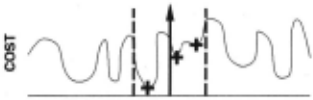
Figure 1: Consider a cost function described over a simple weight space. Assuming the initial value of the weight parameter falls between the two dashed lines, the only local minima that can be reached by gradient descent are those marked with crosses ( + ), even though many other local minima may exist.
must be independent. The problem, of course, is how to achieve "independent" networks. In order to achieve independence in networks, one would expect to have to greatly vary a number of aspects of the networks in cluding (but not limited to) the set of training patterns, the topology of the networks, the learning parameters of the networks, and the method for initializing the net works. But we have investigated a method that empiri cally produces good results for combining networks that only requires the user to vary the method of initializ ing the networks. We do not mean to claim that the resulting networks are truly independent, merely that the networks initialized as we suggest are less interde pendent that networks initialized in the normal manner, and therefore more effective when used in combination.
Our idea is to initialize the parameters, (i.e., weights and biases) of a neural network over a much larger range of values than normal. We do this to cause backprop agation to seek local minima not normally encountered using standard initialization (see Figure 1) .
We explored a number of means to achieve our goal of a diverse set of starting points in weight space; the best one is a method employing competitive learning [Rumelhart and Zipser, 1985] to produce class pro totypes that are used as hidden units in a network in a method similar to Moody and Darken's [1988; 1989] . In Section 3 we outline competitive learning, and in the following section we discuss how to use it to ini tialize neural networks. Section 5 shows experiments we performed on two real-world data sets, demonstrating the advantages of our approach. We then discuss future research directions, related work, and our conclusions.
2 Combining Multiple Networks
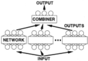
The basic idea in combining neural networks is to train a number of networks, and then somehow use the collec tion to increase generalization. Figure 2 shows a frame work for combining multiple networks.
The choice of a function for combining predictions is important [Kearns and Seung, 1995]. Examples of com bination functions include votin~ schemes [Hansen and Salamon, 1990], simple averages lLincoln and Skrzypek, 1990], weighted average schemes [Perrone and Cooper, 1994; Rogova, 1994], and schemes for training combin ers [Rost and Sander, 1993; Wolpert, 1992; Zhang et al., 1992]. We chose as our method for combining networks the scheme of simply averaging the values of the cor responding outpi.tt units . Results from portfolio theory suggest this method provides a good solution with min imal extra work [Mani, 1991] .
Hansen and Salamon [1990] explored the value of com bining multiple networks. They demonstrated that un der certain assumptions, generalization will increase as more networks are combined. For each pattern where the average error rate is less than 50% for the possi ble trained networks, Hansen and Salamon demonstrate that in the limit the expected error on that pattern can be reduced to zero. Of course, since not all patterns will necessarily share this characteristic (e.g., outliers may be predicted at more than 50% error), the error rate over all the patterns cannot necessarily be reduced to zero. But if we assume a significant percentage of the patterns are predicted with less than 50% average error , gains in gen eralization will be achieved. A key assumption of Hansen and Salamon's analysis is that the networks combined should be independent in their production of errors.
Typically, the weights of a neural network are ran domly initialized with small values. The problem with this approach is that this tends to confine the explo ration of the network to a single area of weight space (Figure 1). Given similar training sets, this means that multiple networks may often find the same local minima. In order to produce networks that are less interdepen dent in their predictions, we investigated methods that avoided this bias. In particular, we focused on chang ing the standard means of initializing network weights to produce networks that have large initial weights .
Our first approach was the obvious solution - use a much larger random range for generating initial network weights. This works well in terms of producing large weights, but the resulting networks suffer from the fiat spot problem [Fahlman, 1988] - backpropagation is un able to refine these networks since the activation values of the hidden and output units tend to be very close to 0 or 1. 2 This occurs because the net input values for a network unit will often be highly positive or negative.
In our second approach we tried to randomly pick ex amples from the training data to act as "prototypes." We then created a hidden unit for each prototype with large positive weights for each of the "on" features of the prototype. This solution also suffered from the flat spot problem, since in a large input space only a small number of examples will share a large set of features with another example and, hence, the hidden units are typically inactive. Using what we learned from this approach, we switched to an approach where we produced hidden units that represented groups of patterns rather than single patterns. Our solution makes use of the tech nique of competitive learning, which we outline next .
2Error is multiplied by activation(! -activation) when backpropagating, assuming a logistic activation function and a sum-of-squared-errors cost function. For units with activa tion near 0 or 1, this means that little error is propagated.
3 Competitive Learning
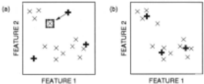
Competitive learning [Rumelhart and Zipser, 1985] is a simple unsupervised learning technique that can be used to partition a set of examples into classes. We start competitive learning by randomly creating a set of class seeds (which are simply points in a feature space). The seeds then compete for the training examples; a seed "wins" an example if it is closest to the example. When a seed wins the competition for an example, the seed is updated by moving it towards that example. Over a number of training epochs, the seeds will move to loca tions in feature space that represent groups (classes) of similar examples (see Figure 3).
We can view competitive learning as a technique to find a set of "seeds" which represent the average member of that class . Each seed j has a value for each input feature i which we will refer to as w; ,j . To calculate the class of an example, we first evaluate a closeness-of-fit metric for each seed, LiEinput· lw; ,j- /;I, where /; is the value of feature i in the example. The seed j with the lowest total difference is the "winner" for the example (i .e., the example is a member of this class) . Learning can be done by changing the average value of input i for the winning seed by an amount t-t(/; - Wi ,winner), where f.l is the learning rate (we used f.l = 0. 01). This process is repeated for each of the examples for a number of epochs (we used 50 epochs) .
4 Combining Networks Initialized via Competitive Learning
Table 1 contains our algorithm for training multiple neu ral networks initialized via competitive learning.
Competitive learning takes a set of examples and par titions it into J classes (where J is user defined). For the following discussion we will refer to the clusters pro duced by competitive learning as subclasses, since each represents a subclass of one of our output categories. We want to create a network that has a hidden unit corresponding to each of the subclasses of each category, where each hidden unit will have an activation near 1 for the examples in its subclass and 0 otherwise. Figure 4 shows a sketch of the resulting network.
Table 1: Algorithm for initializing [( networks using competitive learning. J is the number of hidden units that will be in the resulting network.
Repeat [( times
Randomly choose J seeds, then use competitive learning to create subclasses for each category of examples Use the subclasses for all of the categories to initialize a neural network
Train the resulting network using backpropagation
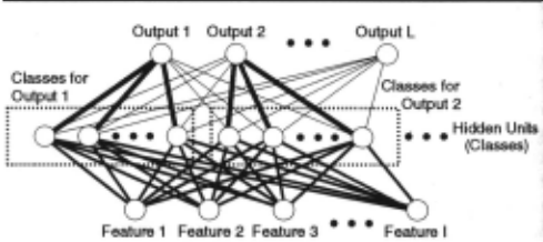
Figure 4: Network combining the results of compet itive learning. Input features are connected to hid den units representing subclasses using weights de termined by competitive learning. Classes are con nected to their output category's unit with a large weight and to other output categories with a small random weight.
In our network we initialize the links between an out put unit and the hidden units representing the subclasses of that category with large positive links (uniformly in [3.9, 4.1]), and set the bias of the output unit so that if any of the subclasses are active, the output unit will be active . We also connect the hidden units associated with a particular output unit to the other output units , using small randomly-weighted links (uniformly in [-0 .1,0.1]); this is done so that backpropagation can use recognizers of subclasses defined for one output category in recog nizing other output categories.
Finally, we have the question of how we create a hid den unit that recognizes a subclass defined by competi tive learning. The weights w; ,j of the seed of a compet itive learning class represent the average feature values of examples in that subclass. If we assume that all of the input features are Boolean 3 , each weight represents how important a particular feature is for an example to be part of that subclass. Recall that we want to create a hidden unit whose weights are dependent on the compet itive learning seed's weights, and which has an average activation value near 1 for examples in that subclass and 0 for others .
The first thing we do is determine the average activa tion value (a) we want the unit to have when it is "on" and similarly for "off." Since we are using the sigmoidal activation function :
we can determine what value of netinput is needed to produce a particular average activation value by solving for netinput in Equation 1. For example, if we want our hidden unit to have an average activation value a of 0.9 when it is "on" we would need netinput = 2.19. Let us assume we have determined the average netinput values net 0n and net off, which are the required netinput values for our desired average activation values.
3 This assumption can be relaxed using a more complex recognition scheme similar to the fuzzy recognition scheme presented by Berenji and Khedkar [1992] .
Next we create a hidden unit that has weights copied from the competitive learning seed. We use this hidden unit to calculate the average net input for the examples that are part of that subclass, and similarly the average net input for examples that are not part of the subclass (call these values avginclass and avgother) . We then cal culate a multiplier m for the weights and a bias b for the unit so that the average net input for the examples in the subclass will sum to net 0 n, and to net off for those examples not in the subclass. To do this we solve for m and b in these equations:
We multiply the hidden unit's weights by m and set its bias to b, making the unit a detector of its subclass. We repeat this process for each subclass of each category, producing a network ready for backpropagation.
Recall that our main goal is to have a set of ini tial networks that are widely dispersed in weight space. The variability of our networks comes from two main sources: (i) we randomly choose the J seeds and (ii) the competitive-learning algorithm randomly sequences through the training examples. (In addition, as ex plained above, we randomly select hidden-to-output weights from small uniform ranges.) Due to computer time limitations, we held the number of seeds constant in our experiments. Varying the number of seeds would increase the variability, and is a topic for future work.
5 Experiments
To judge the value of combining neural networks, we contrast four approaches:
- single network - train a single network. This ap proach is meant to represent methods that do not use multiple neural networks.
- minimal train error - train K networks, selecting the network that does the "best" on the training data. This is an obvious approach to using multi ple networks - select the network that does best on the training data on the assumption that the same network will be the best on the test data.
- oracle - train K networks, selecting (using an or acle) the network that generalizes best. This ap proach cannot be applied in practice because there is generally no oracle that can indicate how general a solution is, but this "approach" will provide a good baseline, since it might appear on the surface that this is the best one can do.
- combination - train K networks and then combine their predictions.
We consider two ways of initializing the networks being trained: (a) the standard approach of randomly selecting weights and biases from a small interval centered on zero; (b) our approach that uses competitive learning.
5.1 Test domains
Our two test domains are a set of handwritten digits from Shen [1992] and the protein secondary-structure data from Qian and Sejnowski [1988] . The first data set contains 3301 8x8 digitized numerals. The problem is to recognize the digit (0-9) in the 8x8 binary image. The second data set has 21 ,623 subsequences of 13 amino acids (each amino acid takes 21 bits to represent, so there are 273 input units) . The output for this problem is one of three categories: whether the central amino acid is part of a helix, sheet, or coil.
5.2 Methodology
We train our networks using a cost function that is the squared-error between the correct and predicted outputs. To mitigate overfitting, for the digit-recognition data we added a sum-of-weight-magnitudes complexity term to the cost function (which is equivalent to using weight de cay [Hinton, 1989]), while for the protein-folding data we used validation sets [Lang et al., 1990] (tests with weight decay produced poor results compared to the standard results for this data set).
However, we did not use the cost function when eval uating the trained networks. Instead, as is typical, we interpret the output unit with the highest activation as the predicted class, and measure testset error by compar ing the predicted class to the correct class. (We also use this methodology to select the minimal-error classifier.)
To measure generalization we performed five 10-fold cross-validation tests on each data set . In 10-fold cross validation, the data is randomly divided into 10 groups . We then create 10 (possibly composite) classifiers for the data- each classifier uses a different one of the 10 groups as test data, and the other nine groups as training data. (Note that we learn only from the training data; the test data is set aside during learning.) We then calculate the testset error for the 10-folds and average over the five runs. For the single-network results our classifier is, naturally, a single network. For the minimal-error clas sifier we train 10 networks and then choose the network that achieves the lowest error on the training set as our classifier. The oracle-based classifier uses the same 10 networks, but it "cheats" by applying the networks to the test data and then using the network that achieves the lowest error on the test data. For the combination results we average the outputs of the 10 networks to ob tain a single prediction.
To initialize the networks for our competitive-learning approach, we run competitive learning for each of the different categories of outputs. For the digit data, we use competitive learning to create five subclasses for each type of digit. Thus there are 50 hidden units (five subclasses for each of 10 digits) in the networks. This number was suggested by other empirical tests on this data set [Cherkauer, personal communication] . For the protein-folding data we used 40 hidden units, which Qian and Sejnowski [1988] concluded was an effective number . We used competitive learning to produce 10 helix sub classes, 8 sheet subclasses and 22 coil subclasses (these numbers reflect the approximate distribution of the data among the three categories of outputs).
| Initialization | ||
|---|---|---|
| Method | Standard | Competitive |
| Single Network | 11.7% | 15.6 |
| Minimal Error | 11.4 | 12.7 |
| Oracle | 9.4 | 9.8 |
| Combination | 9.7 | 8 .8 |
| Initialization | ||
|---|---|---|
| Method | Standard | Competitive |
| Single Network | 37.8% | 35.9 |
| Minimal Error | 38.0 | 36.0 |
| Oracle | 34.7 | 34.3 |
| Combination | 34.9 | 33.8 |
5.3 Results
Our results appear in Tables 2 and 3. For each of our tests we report four pairs of numbers: one for the stan dard backpropagation method of initialization (Stan dard) and one for our method of initialization (Compet itive) . For each data set , we always used networks with the same number of hidden units. The testset error rates reported correspond to the four approaches listed above: using a single network; 4 choosing, from the 10 networks, the network that is most accurate on the training data; choosing the network among the 10 that is most accurate on the testset; and using (for each example) the mean prediction of the 10 networks.
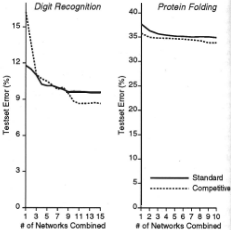
For both data sets the best result was achieved by our combination of networks initialized using competi tive learning, even though the individual networks did not necessarily perform well. The reduction in error for our combination of networks using competitive learning (Combination/Competitive) compared to the standard approach of training a single standard neural network (Single-Network/Standard) is statistically significant at the p < 0.05 level (i .e., with 95% confidence) for both sets of data. Apparently the networks initialized with competitive learning are more independent in the errors, since in combination they lead to decreases in testset error . An interesting point to note is that the combina tion results for our approach are better than the oracle results - even though the oracle may seem to be ideal.
As a baseline for comparison, note that the best re ported error rate for the digit-recognition task is 14.9%, using decision lists [Shen, 1992]. For this set of protein folding data, the best reported error rates are 37.3% using; standard neural networks [Qian and Sejnowski, 1988j, 36.6% using a knowledge-based neural network [Maclin and Shavlik, 1993], and 30.7% using a case-based reasoning algorithm (and a somewhat larger data for mat) [Leng et al., 1994] . Our results are better than all but the case-based reasoning results (which also used a different input encoding).
In Figure 5 we report error as a function of the number of networks combined. As one might expect, the error shows a sharp drop when combining the first few networks and then a gradual .decrease. One general conclu sion is that combining the predictions of several neural networks is a wise decision; doing so is algorithmically simple and can lead to sizable reductions in testset er ror compared to the traditional approach of using one trained network. This reduction holds even if one does not employ our approach to initializing networks.
4 We report the average error rate of the 10 networks.
6 Future and Related Work
We plan to study a number of other methods for creating independent networks. 5 Other methods we would like to try include varying the network architecture (the num ber of hidden units), using different training sets , and varying other training parameters (such as the learning rate). We also intend to study the question of how to determine the optimal number of networks to use in a combination. Finally, we plan to design a scheme for fil tering out networks - some means to recognize networks that are likely to hurt performance.
A number of areas of research are related to the work we presented in this paper . Combining predictions has a long history in a number of fields (for an overview in the area of forecasting see Granger [1989]). In the field of neural networks, a number of researchers have looked at the advantages of combining multiple predictions. Lincoln and Skrzypek [1990] and Hansen and Salamon [1990] both explore the advantages of combining groups of networks in a simple way. Many researchers [Ghosh et al., 1992; Hashem et al., 1993; Perrone and Cooper , 1994; · Rogova, 1994; Wolpert, 1992] have studied the problem of combining predictions in a more robust way, taking into account the confidence of the prediction. Another solution to this problem is to use a learning system, such as neural networks , to learn how to combine the results of multiple predictions. Zhang et al. [1992] and Rost and Sander [1993] use this method. Jacobs et al [1991] have taken the approach of combining multiple networks one step further, in that they attempt to evolve a set of subnetworks such that each subnetwork is good at pre diction for a different region of input space.
5 The main difficulty in pursuing these other experiments is CPU time; our protein folding experiments required us to train 500 networks (5 random repeats of 10 networks for each of 10 cross-validation folds), and each of these networks takes a little more than 1 CPU day of training.
A related approach to our method of choosing various starting points in weight space is to vary the training process to produce networks that are independent and therefore useful for combination. Examples of this ap proach include Reilly et al. 's multi-resolution architec tures [1987], Schapire's [1990] and Drucker et al.'s [1994] boosting algorithms, Hampshire and Waibel 's [1990] use of different objective functions, Baxt's [1992] method of training networks on different tasks, and Perrone's [1992] tree-structured neural networks.
Our method of combining competitive (unsupervised) and backpropagation (supervised) learning is similar to a number of other approaches [Hecht-Nielsen, 1988; Huang and Lippmann, 1988; Moody and Darken, 1989]. The main difference between our work and this previous research is that we use a hybrid unsupervised/supervised network as a method for producing networks that are very effective when used in combination, while the oth ers focused on producing a better single network.
Although we were not aware of the close relationship when we developed our algorithm, our approach is sim ilar to Moody and Darken's [1989] . However, our goals were different from theirs: we wanted to produce net works with large initial weights, while their focus was on partitioning the input space. Our method differs from Moody and Darken's in that we employ standard sig moidal units rather than Gaussian units, and after our initialization phase we use supervised (backpropagation) learning throughout the network, rather than just be tween the hidden and output layer. Our work is also closely related to Nguyen and .Widrow's [1990] which initializes a set of hidden units to each be responsible for a different region of input space; the main difference is that in our work we use competitive learning and our examples to select these regions rather than trying to select them randomly.
Our work also relates to hybrid systems that mix lev els of unsupervised and supervised learning in neural networks [Hecht-Nielsen, 1988; Huang and Lippmann, 1988] . One difference in our work is that we perform our unsupervised learning among the categories separately. We also transform the results from competitive learn ing using our weight multiplier - producing large initial weights. Finally, we install the results of competitive learning into a standard network, so that we can use backpropagation to adjust the resulting subclasses.
7 Conclusions
A fundamental goal for inductive learners is to gener alize well - that 1s, produce classifiers that accurately predict future examples. We present a straightforward approach for improving generalization in which we combine the predictions of several separately trained neural networks . To be productively combined, each individ ual network should represent solutions whose errors are largely independent of those of the other networks. Our key idea is to use competitive learning to initialize our networks . Using competitive learning allows us to cre ate initial networks that lie far from the origin in weight space, .yet do not suffer from the "flat-spot" problem that can greatly slow backpropagation training; thus , we are capable of reaching a wider variety of the local minima in this space than are reachable by the standard network initialization method.
The first step in our network-initialization algorithm is to use competitive learning to cluster the input pat terns for each category into subclasses of that category. In our second step, we create a neural network where each subclass is recognized by one hidden unit . Finally, we perform backpropagation to refine the resulting net work. We repeat this process a number of times to create several networks that in combination generalize well, ac cording to our experiments on two real-world testbeds.
While we are not the first to make the point that the "train-multiple-classifiers" approach is useful, our exper iments do provide additional evidence of the merit of this simple technique for improving generalization. In addi tion, we present a novel algorithm that improves one important aspect of this task, namely the initialization of the set of networks to be trained.
@inproceedings{ijcai1995p69,
  title     = {Combining the Predictions of Multiple Classifiers: Using Competitive Learning to Initialize Neural Networks},
  author    = {Maclin, Richard and Shavlik, Jude W.},
  booktitle = {Proceedings of the Fourteenth International Joint Conference on
               Artificial Intelligence, {IJCAI-95}},
  publisher = {International Joint Conferences on Artificial Intelligence},
  editor    = {Chris S. Mellish},
  pages     = {524--530},
  year      = {1995},
  note      = {Connectionist Models},
  url       = {https://ijcai.org/proceedings/1995/69},
}
TY - CPAPER TI - Combining the Predictions of Multiple Classifiers: Using Competitive Learning to Initialize Neural Networks AU - Maclin, Richard AU - Shavlik, Jude W. T2 - Proceedings of the Fourteenth International Joint Conference on Artificial Intelligence, IJCAI-95 PB - International Joint Conferences on Artificial Intelligence PY - 1995 SP - 524 EP - 530 UR - https://ijcai.org/proceedings/1995/69 ER -Copied
Machine-readable versions of this paper, for tools and AI agents:





