
k-Best: A New Method for Real-Time Decision Making
Proceedings of the Fourteenth International Joint Conference on Artificial Intelligence. Automated Reasoning. Pages 227-234.
© 1995 International Joint Conferences on Artificial Intelligence
Abstract
Many real-world problems, such as air-traffic control and factory scheduling, require that a sequence of decisions be made in real time. The real-time constraint means that we typically do not have sufficient time to find a complete solution to the problem using traditional methods before we must commit to a decision. We propose an incremental search approach to making real-time, sequential decisions, and then present a new decision method called k-best, which is both an extension of an existing realtime decision method (MINIMIN) and an approximation to a decision-theoretic approach to the real-time decision problem. We next provide an analytical bound on the worst-case expected error when k-best is used instead of the optimal decision method. The averagecase performance of k-best is then compared to MINIMIN on a set of randomly generated problems. Our results show that k-best is an improvement over MINIMIN, although MINIMIN performs quite well. Given that MINIMIN is very efficient and easy to implement, we conclude that it should .be the algorithm of choice for many real-time decision problems.
- [Dean and Boddy, 1988] Thomas Dean and Mark Boddy. An analysis of time-dependent planning. In Proceedings, Seventh National Conference on Artifi- cial Intelligence {AAAI-88) , St. Paul, MN, pages 49- 54, Palo Alto, CA, 1988.
- [Horvitz, 1990] Eric J. Horvitz. Computation and Ac- tion Under Bounded Resources. PhD thesis, Stanford University, December 1990.
- [Korf, 1990] Richard E. Korf. Real-time heuristic search. Artificial Intelligence, 42(2-3):189-211, March 1990.
- [Mutchler, 1986] David Mutchler. Optimal allocation of very limited search resources. In Proceedings, Fifth National Conference on Artificial Intelligence ( AAAI- 86), Philadelphia, PA, pages 467-471, Palo Alto, CA, 1986.
- [Pemberton and Korf, 1994] Joseph C. Pemberton and Richard E. Korf. Incremental search algorithms for real-time decision making. In Proceedings, Second In- ternational Conference on Artificial Intelligence Plan- ning Systems {AIPS-94), pages 140-145, 1994.
- [Russell and Wefald, 1991] Stuart Russell and Eric We- fald. Do the Right Thing. MIT Press, Cambridge, MA, 1991.
- [Shannon, 1950] C. E. Shannon. Programming a com- puter for playing chess. Philosophical Magazine, 41(7):256-275, 1950.
- [Zhang and Korf, 1995] Weixiong Zhang and Richard E. Korf. Performance of linear-space search algorithms. to appear in Artificial Intelligence, 1995.
References were extracted automatically from the PDF and may contain errors.
Full text extracted automatically from the PDF; figures, tables and equations may differ. The PDF is the version of record.
1 Introduction
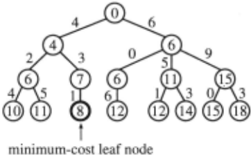
One example of real-time decision making is factory scheduling when the objective is to keep a bottleneck resource busy. In this case, the amount of time available to decide which job should be processed next is limited by the time required for the bottleneck resource to pro cess the current job. Once a new job is scheduled, the time until the new job finishes processing can be used to decide on the next job. In general, this class of problems requires the problem solver to incrementally generate a sequence of time-limited decisions. This consists of three sub-parts: gathering information (e .g., what jobs need to be processed), deciding when to stop gathering infor mation (i.e., what the decision deadline is), and making a decision based on the available information (e.g., what job to process next). For this paper, we have focussed on the last question, namely how to make decisions based
3 The Incremental Decision Problem
We begin by describing the last incremental decision problem, which is a simplified version of the general in cremental decision problem. An example of a last incre mental decision problem is shown in Figure 2. In this fig ure, the black edge costs (z1, z2, Yt, Y2, Ya, Y4) are known, and the grey edge costs ( z1 , . .. , zs) are independently cho sen at random from a known distribution. The decision task is to choose a child of the current root node so that the expected cost of a complete root-to-leaf path is min imized. After we choose a child of the current root node, then we can expand the frontier nodes below that child, and learn the remaining edge costs in the chosen subtree, before making the remaining decisions. The last incre mental decision problem is basically a choice between a set of partially explored subtrees in which we will subse quently execute a sequence of optimal decisions.
The general incremental decision problem is just an extension of the last incremental decision problem to an arbitrary number of decisions. The main advantage of studying the last incremental decision problem over the general incremental decision problem is that we know that the remainder of the tree will be explored after the decision is made. This means that the distribution of minimum-cost paths that will be traversed below a given child of the root node is the same as the distribution of minimum-cost paths in the tree below that child, inde pendent of the decision and exploration methods. This is why we have focussed our efforts on the last incremental decision problem.
4 Making a Last Incremental Decision
Consider the last incremental decision problem shown in Figure 2. The top two levels have been explored, and the bottom level of the tree (the gray edges and nodes) has not been explored. At this point, we must choose between nodes B1 and B2 . We know that the remaining edge costs are chosen independently from a uniform dis tribution over [0, 1], and that once we make a choice, we will be able to explore the remaining edge costs in the chosen subtree before making any additional decisions. The reader is encouraged to stop and answer the follow ing question: Should we move to node B1 or node B2? The obvious answer to this question is to move toward B1 because it is the first step toward the lowest-cost frontier node (node_cost(Ct) = .49 + .3 = .79). This decision strategy, which is called minimin decision making in [Korf, 1990j (or simply MINIMIN), has been employed by others for single-agent search (e.g., [Russell and We fald, 1991]), and is also a special case of the two-player minimax decision rule [Shannon, 1950].
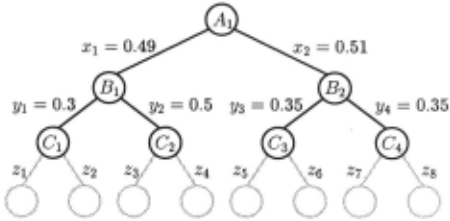
In fact, the optimal decision is to move to node B2 be cause it has a lower expected minimum root-to-leaf path cost. The expected minimum root-to-leaf path cost (or simply expected minimum path cost) through either B1 or B2 is the equal to the. edge cost between the root and the child node plus the expected cost of the path that will be traversed after the remaining edge costs are learned. To make an optimal last incremental decision (and to show that B2 is the better decision in our exam ple), we must calculate the expected minimum path cost through both children of the root node given the edge costs in the explored tree and the edge-cost distribution for the unexplored edges.
In order to calculate the expected minimum path cost for a child of the root node, we need to first calculate the distribution of minimum path costs for that child node. In general, the problem of calculating the distribution for a minimum-cost path from a child of the root node to a leaf node can be broken down into two steps. The first step is to determine the distribution for a minimum-cost path from a frontier node to a leaf in the tree. The sec ond step is to combine the frontier node completion-cost distributions with the known edge costs in the explored search tree.
For node C1 in Figure 2, there is one unexplored level between the frontier node ( cl) and the leaf nodes below it . The cumulative distribution Fe, (z) can be calculated as follows (F(z) = z is the edge-cost distribution). We assume that the edge-cost distributions are independent.
Given the distribution for a minimum-cost path from a frontier node to a leaf node, the second step is to cal culate the expected minimum path cost through a child of the root node. This involves constructing a piece wise combination of the frontier-node minimum-path cost cumulative-distribution functions ( CDF's ). Figure 3 shows the CDF's for frontier nodes C1 and C2 as well as the combined CDF for node B 1 for two differ ent relative values of y1 and Y2 (Fcc( Ct) = Fe, (z- yt), Fcc(C2) = Fc,(z- Y2)).
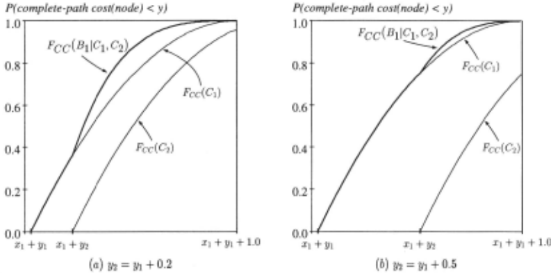
Finally, the cumulative-distribution functions for the children of the root node (i.e., B1 and B2) are differen tiated to yield the probability density functions (PDF's) for minimum path cost through these nodes. These PDF's are then used to calculate the expected minimum path costs through each child of the root by integrating over the range of possible root-to-leaf path costs. The optimal last incremental decision is then to move to the child with the lowest expected minimum path cost.
We can now return to the example in Figure 2. If we assume without loss of generality that Yl :::; Y2, then the equation for the expected cost of a complete path through node B 1 is:
An analogous equation applies for node B2 . Sub stituting the edge costs from Figure 2 into Equation 1, we get E(min_path_cost(Bt)) = 1.066, whereas E(min_path_cost(B2)) = 1.06. Thus node B2 is the optimal decision for this example. Intuitively, a move to node B1 relies on either z1 or z2 having a low cost, whereas a move to B2 has four chances (zs, z6, Z7 and z8) for a low final edge cost. Thus, an optimal last in cremental decision is a move toward the child node with the lowest expected root-to-leaf path cost that will be traversed after the incremental decision is made and the remaining edge costs are learned.
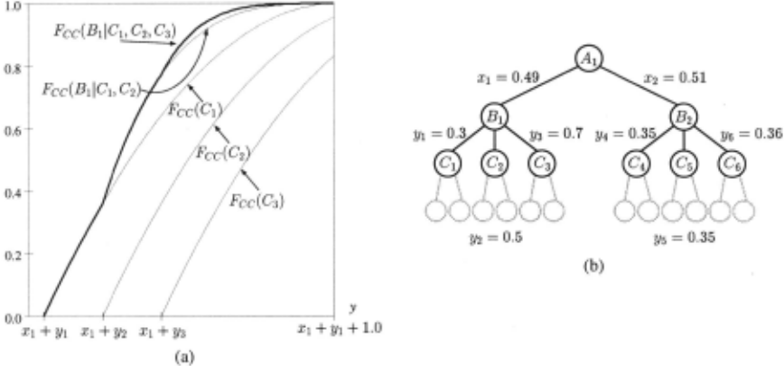
In general, finding an optimal last incremental deci sion is impractical for all but a few small search trees. The difficulty comes from the fact that the distribution of minimum path costs through a child of the root can have a distinct distribution function for each frontier node in the child node's subtree. For example, consider the graph and tree shown in Figure 4. This tree has one more frontier node under B1 than our original example (Fig ure 2). The graph shows the cumulative distribution of minimum root-to-leaf path costs through nodes Ct, C2 , C3 , and B1 versus the cost of a path to a leaf node. We observe that each of the three frontier nodes under B1 is responsible for a change to the minimum-path-cost dis tribution for B1 (Fcc(Bt)). For example, the change in the distribution at y = z1 + Y2 is due to the fact that at first every minimum-cost path through B1 must also pass through C1 . Once the minimum path cost is greater than or equal to z1 + y2 , then a minimum-cost path be low B1 can be through either C1 or C2 · This additional choice causes a sharp rise in the cumulative distribution function for B1 at z 1 + y2 , as shown in the graph. Since the number of frontier nodes in each subtree is exponen tial in the search depth, in the worst case the number of different functions needed to describe the minimum path-cost distribution is also exponential in the search depth. This is why calculating the expected minimum root-to-leaf path cost and consequently making an opti mal last incremental decision is only possible for a set of small search trees.
Thus far , we have presented two disparate incremental decision methods: MINIMIN, which is easy to calculate but makes suboptimal decisions, and the optimal deci sion strategy, which only works on small search trees. In the next section, we present a new decision method that bridges the gap between MINIMIN and the optimal decision method.
5 k-Best: A New Incremental Decision Algorithm
k-best is a new algorithm for making incremental deci sions. It operates by maintaining a list of the k-best frontier nodes under each child of the root node as the subtrees are explored. These k-best frontier node costs are then used to calculate an approximation of the ex pected min;,,l.um root-to-leaf path cost for each child of the r<· · · r.ode. The approximation is calculated by as sL.ming that the child's subtree only contains the k-best frontier nodes. The k-best decision is simply to move to the child with the lowest k-best estimate of the expected minimum root-to-leaf path cost.
Consider again the tree shown in Figure 4b. First, we observe that the the lowest-cost leaf node ( Ct) un der a given child of the root node has the greatest ef fect on the distribution of minimum-cost paths through that child because it determines the starting point of the minimum-path-cost distribution (i.e., Fcc(Bt) initially equals Fcc( Ct) because C1 is the lowest cost frontier node). The next largest effect is due to the location of the second-best frontier node (C2 ) in a child's subtree, and the size of the effect diminishes as we approach the highest-cost frontier node. For example, when the mini mum root-to-leaf path cost through B1 becomes greater than or equal to z1 + y2 , then the distribution of mini mum path costs for B1 shifts to a new function that com bines the distributions of minimum path costs through C1 and C2. When the minimum path cost through B1 is greater than or equal to z1 + Ya, then the minimum path-cost distribution for B1 shifts again to reflect the third frontier node, although the size of the second shift is much smaller than the first shift. In fact, it is of ten the case that the higher-cost frontier nodes under a given child node do not contribute at all to the distribu tion of minimum-cost path through that child because their node cost exceeds the minimum frontier-node cost by more than the maximum possible edge cost.
k-best takes advantage of this observation by simply ignoring all but the k-best frontier node costs below each child of the root node. To make k-best tractable, we sim ply choose a value for k that is small enough so that we can calculate the expected minimum-path-cost equation. When k = 1, k-best and MINIMIN will make the same decisions (up to tie-breaking). Alternatively, when the number of frontier nodes in each subtree is less than or equal to k, then k-best makes optimal last incremental decisions. Thus k-best defines a continuum of decision algorithms between MINIMIN and the optimal decision method.
The obvious question at this point is what is the cost in terms of solution quality of this approximation? The worst-case expected error for a k-best decision occurs when k-best chooses a decision that only has k good frontier nodes, and all the frontier nodes below the deci sion that wasn't chosen by k-best are good, in the sense that their node costs are very close to (or perhaps equal to) the minimum frontier-node cost. This is the situa tion where the optimal incremental decision has greatest potential advantage over k-best. An example of this sit uation is shown in Figure 5, where f is a small constant .
For this example, the k-leftmost frontier nodes all have cost z, which is the minimum frontier-node cost, and the other m- k frontier nodes below node B1 have node costs equal to z + 1, which is equal to the minimum frontier-node cost plus the maximum edge cost. This means that only these k minimum-cost frontier nodes can contribute to the expected minimum path cost below B1 . We assume that there are m frontier nodes below B2, all of which have a node cost equal to z +f. We also assume that there is one remaining unexplored level of the tree and that the branching factor in this level is b.
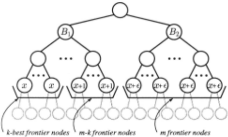
The expected error of a k-best decision is simply the difference between the expected minimum path cost be low the k-best decision (BI), and the expected minimum path cost below the optimal decision (B2). For simplic ity, we assume that the unexplored edge costs are inde pendently chosen from a uniform distribution over the range [0, 1] (i.e., F(z) = z (0 ~ z ~ 1)). Since the k minimum-cost frontier nodes are the only frontier nodes that can appear on a minimum-cost path below Bt, the expected minimum path cost below B1 is equal to z plus the expected cost of a minimum choice between kb ran dom edge costs. For this edge-cost distribution, the ex pected cost of a minimum choice between kb random edge costs is 1/(kb + 1).
In order to calculate the expected minimum path cost below B2 , we simply observe that the optimal decision after moving to B2 will be a choice between mb edge costs added to one of the m frontier nodes that have cost z +f. For this edge-cost distribution, the expected value ofmb random choices is 1/(mb+ 1). Thus the expected minimum path cost below B2 is z + f + 1/(mb + 1).
The worst-case expected error for a k-best decision, on this example problem, is simply the difference between these two expected minimum path costs. In the limit as m goes to infinity and f goes to zero, this difference approaches 1/(kb+ 1), which is the expected completion cost for the path below a set of k minimum-cost frontier node. This make sense, because as the number of frontier nodes below B2 increases, it becomes more likely that a zero-cost edge will be generated.
Thus the worst-case expected error for k-best on a last incremental decision problem is bounded by the ex pected cost of a choice between kb unexplored edges. This expected-cost bound is a decreasing function of k. In addition, the amount of information that can be gained ask is increased is also a decreasing function of k. Intuitively, it seems reasonable that the most important piece of information about a root-child decision subtree is the minimum frontier-node cost, and the second most important piece of information is the second smallest frontier-node cost, etc.
6 Experimental Comparison of k-best and MINIMIN
In order to compare the average case performance of k best and MINIMIN, we performed a set of experiments on random trees with fixed branching factor, and with edge costs that are independently chosen from the set {0, 1/r, 2/r, ... , (r- 1)/r; r = 1024}. A value of 7 was chosen for k to make the k-best equations manageable. For each trial, random values were assigned to each edge of the problem-space tree, and then both MINIMIN and 7-best were allowed to explore the problem space using a depth-first branch-and-bound exploration up to one level above the bottom of the problem-space tree. This is a last incremental decision problem with one unexplored level. After the MINIMIN and 7-best decisions were cal culated, the remainder of the tree was explored in order to optimally complete both paths. In addition to the 7-best and MINIMIN path costs, we also calculated the optimal path cost in the completely explored problem space tree. We then recorded the percent solution-cost error, calculated as follows.
We also compared the solution cost of the two algo rithms, and recorded. the number of times that each al gorithm produced a lower-cost solution.
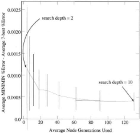
The graph in Figure 6 shows the difference in aver age solution cost error for MINIMIN and 7-best. The vertical axis is the difference between the average MIN IMIN percent solution-cost error and the average 7-best solution-cost error, whereas the horizontal axis is the average generations used per decision for search depths ranging from 2 to 10. Each data point is an average of 10,000 trials, and the vertical line at each point in dicates the 95% confidence interval. The results show that 7-best produces solutions with lower average per cent error than MINIMIN. Although the improvement of 7-best over MINIMIN is very small, it is consistent over the range of random-tree problems considered. The results in Table 1 shows the percentage of the trials that either 7-best or MINIMIN produced a lower cost solution (i.e., wins a head-to-head competition), for the same set of experiments (with 95% confidence intervals). We note that 7-best wins more of the head-to-head competitions than MINIMIN for a given search depth. Although the percentage wins by 7-best is only slightly higher than the percentage wins by MINIMIN, this difference is also consistent over the range of random-tree problems con sidered.
| Search depth | 7-best %wins | MINIM IN %wins | ratio |
|---|---|---|---|
| 1 | 0.0 ± 0.00 | 0.0 ± 0.00 | - |
| 2 | 1.7 ± 0.08 | 1.5 ± 0.07 | 1.133 |
| 3 | 1.9 ± 0.08 | 1.7 ± 0.08 | 1.117 |
| 4 | 2.0 ± 0.09 | 1.6 ± 0.08 | 1.250 |
| 5 | 1.9 ± 0.08 | 1.5 ± 0.08 | 1.267 |
| 6 | 1.9 ± 0.08 | 1.5 ± 0.08 | 1.267 |
| 7 | 1.8 ± 0.08 | 1.5 ± 0.08 | 1.200 |
| 8 | 1.8 ± 0.08 | 1.5 ± 0.07 | 1.200 |
| 9 | 1.8 ± 0.08 | 1.4 ± 0.07 | 1.285 |
| 10 | 1.8 ± 0.08 | 1.4 ± 0.07 | 1.285 |
7 Making a Series of Decisions
Up to this point we have only considered the last in cremental decision problem. We have also applied our k-best algorithm to the problem of making a series of incremental decisions. For a sequence of decisions, we can't guarantee that we will be able to see the bottom of the problem-space tree before the next decision, and thus the completion-cost distribution that we developed for the last incremental decision problem no longer accu rately reflects the situation that will exist for the next de cision. Instead, the distribution of minimum-cost paths that might be traversed below a frontier node will de pend on the decision-making algorithm, the exploration algorithm, as well as the factors that affect the last in cremental decision. For these reasons, and the fact that an optimal solution to the general incremental decision problem will be at least as complicated as the optimal last incremental decision problem, we have assumed that it is reasonable to model the general incremental decision problem as if it were a last incremental decision problem with one additional level of unexplored problem-space tree below the bottom of the search tree.
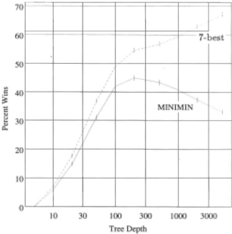
To compare MINIMIN and k-best on a series of deci sions, we performed a new set of experiments where we fixed the search depth of the branch-and-bound explo ration and increased the number of incremental decisions (i.e., the depth of the tree) . Figure 7 shows the percent wins (MINIMIN against 7-best) versus the log of the tree depth for a fixed search depth of 5 on a binary tree (with 95% confidence intervals). The results are averaged over 10,000 trials, and show that as the number of decisions increases (i.e., the tree depth), the percent age of the trials that each algorithm wins initially grows. This makes sense because the number of opportunities for the algorithms to make a different choice increases with the number of decisions. What we didn't expect is that for more than about 300 decisions, the percentage of the trials in which k-best produces a lower-cost solution than MINIMIN continues to grow, at the expense of the percentage of the trials in which MINIMIN produces a lower-cost solution. This result clearly shows that k-best makes better quality decision on average than MINIMIN.
8 Related Work
The results presented here is an extension of our previ ous work reported in [Pemberton and Korf, 1994). Our initial work was motivated by Mutchler's analysis of how to spend scarce search resources to find a complete so lution path [Mutchler, 1986). Our work is also related to Russell and Wefald's work on DTA * [Russell and We fald, 1991), although they have not directly addressed the last incremental decision problem. Eric Horvitz [Horvitz, 1990) has also investigated the problem of reasoning un der resource constraints, which he called flexible com putation. The MINIMIN decision method was initially employed by RTA * [Korf, 1990) and is a special case of the minimax decision rule that is widely used in game tree evaluation [Shannon, 1950).
The main difference between anytime algorithms [Dean and Boddy, 1988) and our real-time incremen tal search algorithms is that anytime algorithms ad dress what we refer to as the complete solution problem, whereas we have focussed on the incremental decision making problem. For example, in the random tree model, an anytime algorithm would generate a complete root-to-leaf path, whereas k-best focuses its attention on improving the quality of the next decision. Thus, instead of generating a complete root-to-leaf path all at once, k best generates the root-to-leaf path one step at a time, while interleaving computation and execution.
In some sense, we can view the computation for each incremental decision as an anytime decision problem. Thus the difference between incremental search algo rithms and anytime algorithms is in the way that the real-time search problem is formulated. Anytime algo rithms try to find the best complete solution under a time constraint, whereas real-time incremental search al gorithms try to find the best next decision under a time constraint.
9 Conclusions
We have presented k-best, which is a new method for making incremental search decisions. We have shown that the expected error of k-best on the last incremen tal decision problem with one unexplored level remain ing is at most equal to the expected cost of the mini mum of kb random edge costs, where k is the number of frontier nodes considered, and b is the branching fac tor of the nodes in the unexplored level of the tree. k best is both an approximation of the optimal decision method, and an extension ofMINIMIN. Our experimen tal results show that k-best decisions are slightly better quality than MINIMIN decisions on average, and that this improvement does add up over long sequences of decisions. Since MINIMIN is easy to implement, and is typically very efficient to execute, we recommend it as the first choice for real-time incremental decision prob lems. When the resource constraint is on the depth of the search rather than the time spent searching (e.g., limited sensor range, unknown future job-scheduling re quirements), then k-best provides a useful way to incor porate additional information about future decisions in order to improve the overall quality of the decision se quence.
Acknowledgements
This research was supported by NSF grant #IRI9119825, the Air Force Office of Scientific Research un der contract 92-0693, ARPA/Rome Labs under contracts F30602-91-C-0036 and F30602-93-C-00031, a grant from Rockwell International, and an equipment grant from Hewlett-Packard. We would like to acknowledge help ful discussions with Rich Korf, Weixiong Zhang, and the members of CIRL. Thanks to William Cheng for tgif, David Harrison for xgraph, and the Free Software foun dation for gee, gdb, and gnuemacs.
@inproceedings{ijcai1995p30,
  title     = {k-Best: A New Method for Real-Time Decision Making},
  author    = {Pemberton, Joseph C.},
  booktitle = {Proceedings of the Fourteenth International Joint Conference on
               Artificial Intelligence, {IJCAI-95}},
  publisher = {International Joint Conferences on Artificial Intelligence},
  editor    = {Chris S. Mellish},
  pages     = {227--234},
  year      = {1995},
  note      = {Automated Reasoning},
  url       = {https://ijcai.org/proceedings/1995/30},
}
TY - CPAPER TI - k-Best: A New Method for Real-Time Decision Making AU - Pemberton, Joseph C. T2 - Proceedings of the Fourteenth International Joint Conference on Artificial Intelligence, IJCAI-95 PB - International Joint Conferences on Artificial Intelligence PY - 1995 SP - 227 EP - 234 UR - https://ijcai.org/proceedings/1995/30 ER -Copied
Machine-readable versions of this paper, for tools and AI agents:





