Representations for Active Vision

1 Introduction: Active Vision Revisited

If Computer Vision was once limited to the study of mappings of a given set of visual data into representa­ tions on a more abstract level, it now has become clear that Image Understanding should also include the pro­ cess of selective acquisition of data in space and time. This has led to a series of influential studies published under the headings of Active, Animate, Purposive, or An important point was missed: that an intelligent vision system exists in space-time (where space-time in­ cludes the system itself) and in order for the system to function properly, i.e., to act appropriately in a variety of situations, it should be able to develop robust descrip­ tions of space-time. That is, it should be able to develop representations that would be adequate for accomplish­ ing a set of tasks. But, classical geometry modeling the 2 1/2-D sketch has been inescapably with us all the time. Recovering the depth of surfaces in view or quantities that are subject of Differential Geometry such as sur­ face normals and curvatures seems to have been about the only goal of 3-D Computer Vision in the past 35 years. During the past few years, however, it has been repeatedly argued that this could be a misplaced goal , simply because it is too difficult to recover such com­ plete descriptions of shape and space [Faugeras , 1992; Koenderink and van Doorn, 1991).

In this paper we propose novel representations of an active observer's space-time and we show how they can be obtained in real time using pattern matching tech­ niques in the spatiotemporal gradients of the image in­ tensity function. The essence of these representations is that they are derived from well-defined input (no corre­ spondence of features is required) and from global com­ putations not affected by local errors of various sorts. In particular, we present new solutions for two basic prob­ lems in Vision, the one of estimating an observer's mo­ tion and the one of recovering a shape description for an active binocular system whose exact extrinsic param­ eters are not known. The next section describes these representations.

2 Retinotopic Motion and Shape Representations

Consider an observer moving in some environment . Al­ though the organism as a whole might move in a nonrigid manner- head, arms, legs and wings undergo different motions-the eyes move rigidly, i.e., as a sum of instan­ taneous translation and rotation. The points where the translational and rotational velocity vectors intersect the retina, called the FOE (focus of expansion), and the AOR (axis of rotation), are respectively the represen­ tation of egomotion. That is, estimation of a system's egomotion amounts to recognizing two locations on the retina.

Similarly, consider a binocular observer fixating on a point in space. The traditional representation used for the observer's extrapersonal space is the depth of fea­ tures in the scene in view, or its derivatives such as shape, curvature, etc. We argue that the shape rep­ resentations to be recovered for an active vision system are different from the metric ones traditionally used in the sense that they cannot provide the 2 1/2-D sketch or functions of it. We call such representations "qualita­ tive structures"; they basically amount to recovering a function of the depth of the scene, where partial informa­ tion about this function is available. More specifically, if z( x, y) is the function providing the depth z at points (x,y) in the image plane, and if/;, i = 1,2, ... ,n is a set of functions not necessarily exactly known, then J;(z(x, y)), i = 1, ... , n is a set of qualitative structures of the scene. For example, iff is a monotonic function in z with the property z(x, y) < z(x', y') {::::=} f(z(x, y)) < f(z(x',y')), then f constitutes a qualitative representa­ tion that we call "ordinal structure," since knowledge about it only allows to order the values of the scene's depth. Functions with different properties amount to qualitative representations of a different nature. In par­ ticular, in this paper we will show that an active binoc­ ular observer not aware of its exact extrinsic parame­ ters capable of fixating at environmental points can re­ cover an ordinal structure of the scene, without relying on the computation of exact correspondence of features in the two images. The concept of ordinal depth com­ putations has its origin in the relief transformations sug­ gested already by the turn of the century psychologist Helmholtz and recently taken up in the work of various perceptual studies [Koenderink and van Doorn, 1991; Todd and Reichel, 1989; Garding et al., 1993] . How­ ever, in these studies either correspondence is assumed or special assumptions are made about the structure of the scene in view.

3 Motion and Stereo Fields and Patterns of Gradients

Most current motion estimation techniques require the computation of exact image motion (optic flow or cor­ respondence of features). This however amounts to an ill-posed problem. On the basis of local information only the component of the optical flow perpendicular to edges, the so-called normal flow, is well-defined, although in many cases, it is possible to obtain additional flow information for areas (patches) in the image. Similarly, the computational analysis of binocular shape percep­ tion has been based on the two-dimensional disparity field , which is a special case of a motion field. In a limited area of the image around the fixation point the disparity measurements are small and thus they can be treated in a differential manner, just as optical flow . As in the case of motion, on the basis of local information only the component of the disparity vector perpendicular to edges, the so-called normal disparity, is well defined. The basic thesis in this paper is the following:

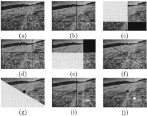
(a) For the case of the motion problem there exists a set of orientation fields on the retina which possess the prop­ erty that measurements of motion available along these orientations have a global structure, i.e., they form sim­ ple patterns whose location and form encode the 3-D mo­ tion parameters. (To obtain an intuition see Figures 1c and d; 3a, band c; and 4a, band c.)

(b) For the case of the stereo problem, there exists a set of orientation fields with the property that measure­ ments of normal disparity that happen to be along these orientations have an ordinal structure regarding depth, i.e., their values are sufficient for ordering the depth of the corresponding scene points (Figure 7a). Mea­ surements in one orientation field allow the derivation of partial ordinal structure. Successive fixations allow the merging of these representations by filling in ordinal depth information from different fixations, thus building up a global ordinal depth map.

4 The Case of Motion: Preliminaries

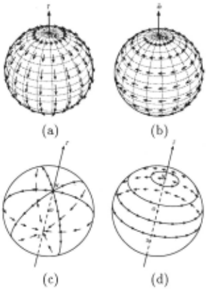
To begin with, let us review the geometry of visual mo­ tion. To obtain a better intuition we first use a spher­ ical retina. If the motion is a translation f, the motion field is along the great circles containing the vector [ (Figure 1a) , pointing away from the Focus of Expansion (FOE) and towards the Focus of Contraction (FOC) . If the motion of the eye is a rotation of velocity w where the rotation axis cuts the sphere at points AOR (Axis of Rotation point) and -AOR, the motion field is along the circles resulting from the intersection of the sphere with planes perpendicular to the rotation axis (Figure 1b). For general rigid motion the motion field on the sphere is the addition of a translational field and a rotational field. However, as input to the motion interpretation process we do not consider the motion field but the sign of the projection of motion vectors on appropriately cho­ sen orientations.

4 .1 Selection of Flow Orientations

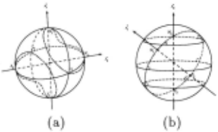
Two classes of orientations are i.ntroduced which are de­ fined with regard to an axis. Consider an axis s pass­ ing from the center of a spherical eye and cutting the sphere at points N and S. The unit vectors tangential to the great circles containing s define a direction for ev­ ery point on the retina (Figure 1c). These orientations are called ?longitudinal. Similarly, the ?latitudinal ori­ entations are defined as the unit vectors tangential to the circles resulting from the intersection of the sphere with planes perpendicular to the axis s (Figure 1d) . At each point the ?longitudinal and latitudinal vectors are perpendicular to each other. Some properties of these di­ rections will be of use later: Consider two axes 81 (N1S1) and 82 (N2S2). Each axis defines at every point a lon­ gitudinal and a latitudinal direction. Figure 2 explains the locus of points where the 81 longitudinal or latitu­ dinal vectors are perpendicular to the 82 longitudinal or latitudinal vectors.

Next, the structure of the projections of a rigid mo­ tion field on the ?longitudinal and latitudinal vectors is examined. More accurately, the sign of the projections of the motion field on the longitudinal and latitudinal vectors is investigated, since this is the information em­ ployed as input to the motion interpretation process. For this purpose it is necessary to agree upon a definition of the directions. 8 (NS) -longitudinal vectors are called positive ( +), if they point away from N, negative (-) if they point away from S, and zero (0) otherwise. Simi­ larly, ?latitudinal vectors are referred to as positive ( +) if their direction is counterclockwise with respect to 8, negative (-) if their direction is clockwise, and zero (0) otherwise.

4.2 The Geometry of Image Motion Patterns

Since a rigid motion field is the addition of a translational and a rotational field, the cases of pure translation and pure rotation are first presented separately.

If the observer moves with a pure translation of ve­ locity f, the motion field on the sphere is along the di­ rection of the {longitudinal vectors (Figure 1a). Pro­ jecting the translational motion field of Figure 1a on the ?longitudinal vectors of Figure 1c, the resulting vectors will be either zero, positive or negative. The vectors will be zero on two curves as shown in Figure 2a (symmetric around the center of the sphere) whose shape depends on the angle between the vectors t and 8. The area inside the curves will contain negative vectors and the area out­ side the curves will contain positive vectors (Figure 3a) .

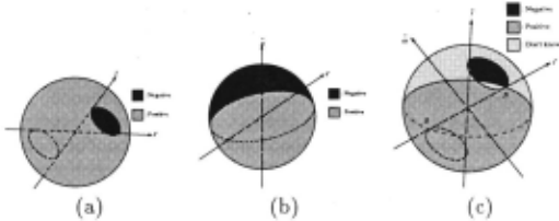
If the observer moves purely rotationally with veloc­ ity w, the motion field on the sphere is along the direc­ tion of the w-latitudinal vectors (Figure 1 b). Projecting the rotational motion field of Figure 1 b on the 8 ( N B)­ longitudinal vectors of Figure 1c, the resulting vectors will be either zero, positive or negative. The projec­ tions will be zero on the great circle defined by 8 and w, positive in one hemisphere and negative in the other (Figure 3b).

If the observer translates and rotates with velocities t and w the projection of the general motion field on any set of ?longitudinal vectors can be classified for parts of the image. If at a longitudinal vector the projection of both the translational and the rotational vectors is pos­ itive, then the projection of the image motion (the sum of the translational and rotational vectors) will also be positive. Similarly, if the projections of both the transla­ tional and rotational vectors on a longitudinal vector at a point are negative, the projection of the motion vector at this point will also be negative. Otherwise the sign will be unknown because it depends on the value of the translational and rotational vector components.

Thus, the distribution of the sign of image motion along the ?longitudinal set of directions defines a pat­ tern on the sphere. Considering a general rigid mo­ tion field due to translation f and rotation w on an s (NS)-longitudinal set of directions, a pattern like the one shown in Figure 3c is obtained, which consists of an area of strictly positive values, an area of strictly neg­ ative values, and an area in which the values can not be determined without more information. The pattern is characterized by one great circle containing w and s and by two quadratic curves containing the points FOE, FOC, Nand S.

It is worth stressing that the pattern of Figure 3c is independent of the scene in view and depends only on a subset of the 3-D motion parameters. In particular, the great circle is defined by one rotational parameter and the quadratic curve by two translational parameters. Thus the pattern is of dimension three. Also, the pattern is different for a different choice of the vector s.

Similarly, considering the projection of a rigid motion field on the Slatitudinal directions (defined by the vector s (N S)), another pattern is obtained which is dual to the one of Figure 3c. This time the translational latitudinal flow is separated into positive and negative by a great circle and the rotational flow by two closed quadratic curves.

4.3 Egomotion Estimation Through Pattern Matching

The geometric analysis described above allows us to for­ mulate the problem of egomotion estimation as a pat­ tern recognition problem. Assume that the system has the capability of estimating the sign of the retinal motion along a set of directions defined by various ?longitudinal or latitudinal fields that happen to be perpendicular to the local edges. (In a number of cases the sign may be estimated in other directions as well). If the system can locate the patterns of Figure 3c in each longitudinal vec­ tor field (and the dual pattern in the latitudinal field), then it has effectively recognized the directions f and w. If information (positive, negative or zero) is not avail­ able in many directions, there might be an uncertainty in the computations in the sense that more than one set of patterns may be fitted to the data and the FOE and AOR may be obtained only within bounds.

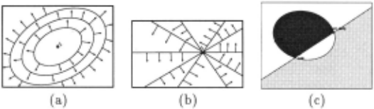
For the case of a planar retina the latitudinal and lon­ gitudinal fields take a different form which is easily com­ puted by projecting them on a plane tangential to the sphere (Figure 4a,b ). In this case areas with negative and positive .normal motion measurements lie in areas separated by a conic section (circle, ellipse, hyperbola, or parabola) and a straight line. Figure 4c pictures an example of a longitudinal pattern. Figure 5 shows re­ sults from experiments on planar images from an out­ door scene.

5 The Case of Fixating Stereo: Preliminaries

Consider an active binocular observer capable of fixat­ ing on an environmental point. The geometry of the system can be described as a constrained rigid motion, between the left and right eye. If we fix a coordinate on the left eye with the z-axis aligned with its optical axis the y-axis perpendicular to the fixation plane, then the transformation relating the right eye to the left is a rota­ tion around the y-axis and a translation in the xz plane (Figure 6) . At the fixation point the disparity measure­ ments are zero and in a neighborhood around it relatively small. Thus, it is legitimate to approximate the disparity measurements through a continuous velocity field. This amounts to the small baseline approximation that has been used in the literature [Garding et al., 1993).

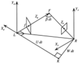
Figure 6: LJ{ = U dt: translation along X1-axis. J{ R = W dt: translation along Z1-axis. LF R = f3 dt: angle denoting rotation around Y1-axis. L, K, R, F belong to the fixation plane. dt is a hypothetical small time inter­ val during which the motion bringing Xt Yi Zt to Xr Yr Zr takes place.

Denoting, as usual, by U and W the translation along the x- and z-axes and by f3 the rotation around the y­ axis, and setting x 0 equal to [{, · f ( x-coordinate of the focus of expansion, where f is the focal length), the com­ ponent Un of the disparity vector (u, v) along the gradi­ ent direction ( nx, ny) is:

The exact geometry of the stereo configuration cannot be assumed and we do not wish to attempt the usual two step approach of first computing it from the available information in order to utilize it and derive in a second step the depth estimates. The reason is that small errors in the parameter estimation of the extrinsic geometry can result in large errors in the depth or shape estimates.

Our approach consists of two steps: (a) First, from one fixation and appropriately utilizing equation (1), we derive a set of partial depth orderings, classes of points for which we know the ordinal depth within each class. (b) From new fixations we obtain new partial orderings, though in different coordinate systems. The fixation ge­ ometry allows us to compare certain values between different fixations. This way we merge values in different fixations and build a global ordinal shape representation.

5.1 Ordinal Depth from One Fixation

An active binocular stereo system capable of changing its geometric parameters in a controlled "-'ay should be aware of the pose of its eyes with regard to some head frame centered coordinate system. Thus it should know the angle the optical axis encloses with the baseline, which amounts to knowing the parameter xo . If for a particular system this knowledge is not available, utiliz­ ing the constraints described in Section 4, the direction of the translation x 0 can be derived from the patterns of the normal disparity field, utilizing only the sign of the disparity measurements.

We do not know, however, the amount of rotation f3 and we also don't have to know the distance between the two eyes. Using equation (1) it is possible to obtain an ordinal depth representation for the scene whose image points lie on families of curves: Dividing equation ( 1) by -nx, we obtain

We now classify normal disparity measurements accord­ ing to their direction as a function of the image coordi­ nates and a constant C. For this reason, we introduce a function g(x, y, xo) such that xo- x- y!:..JL = g(x, y, xo) n, and (f +X/+ y~) = C;g(x,y,xo) for some scalar ci. This defines at each image point ( x, y) a direction for the gradient ( nx, ny)

That is, if at a point ( x, y) the gradient ( nx , ny) is de­ fined by equation (3) as a function of (X, y) and Ci, equa­ tion (2) can be written as:

This result can be given the following geometric in­ terpretation: equation (3) for every C; defines the nor­ mals for a family of curves on the image. Each family of curves is defined by the following differential equation:

where

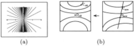
with q = 4 - 4 ~xo - C2 and K an arbitrary constant. Figure 7a shows such a family for C; = 0.2, f = 1, xa = 1. Different C; 's provide different classes of curves. All points with the gradient perpendicular to the curves of one family can be ordered according to their depth.

5.2 Merging of Results from Different Fixations

A new fixation is obtained by rotating the left and the right eyes around the centers of their coordinate sys­ tems (their nodal points). Under a rotation the coordinates of every point Xold = (Xold, Yold, Zold) in the original coordinate frame are related to the coordinates Xnew = (Xnew, Ynew, Znew) in the new coordinate frame after fixation through the linear transformation ~ - ~ T - . Xnew = R·Xold (or Xold = R ·Xnew), where R IS a 3 X 3 rotation matrix, with coefficients rn, r12, ... , 1'33 (and RT the transpose of this matrix). The Z-coordinates Znew and Zold in the two different frames are thus re­ lated as follows:

Points in the original image, whose coordinates are de­ fined by a line equation

where ]{ is a constant, are mapped to lines defined by the equation

in the new image coordinate system.

For any two points (A, B) on these lines the ratio of their depth values is preserved under rotation. That is, if ZAold and ZBold are the depth values associated with the corresponding image point Aold, Bold in the original coordinate system and ZAnew and ZBnew are the depth values of the corresponding image point Anew, Bnew then

This relationship allows us to merge ordinal depth maps from different fixations: In the new coordinate system (new fixation) we obtain a number of partial orderings for classes of points to be found on families of curves (as described in 5.1). Let us consider any such family of curves and let us intersect these curves with the lines defined by equation (8). For any new points to be found on the intersection of a line and one family of curves the ordinal depth relation obtained in the new coordinate system can be utilized to increase the knowledge about the ordinal depth maps in the original frame (see Fig­ ure 7b). Let Cnew and Dnew be two points with gradients perpendicular to the curves of one family and also lying on one line. These points correspond to Cold and Dold in the old coordinate system. Cold belongs to one family of curves and Dold to (usually) another family of curves in the old coordinate system Thus the depth measurements of Cold and Dold could not be compared using only one fixation. Since however , we know the ordinal depth in the new coordinate system and we also know the ratio of differences between a pair of points in the two coordinate systems, we can increase the number of points with or­ dinal depth information of the family of curves on which Cold lies, by the point Dold. Similarly, we can increase the number of points of the family containing Dold, by the point Cold [Fermi.iller and Aloimonos, 1995]. Any two measurements in the new coordinate system which lie on a straight line (given by equation (7)) and on the curves of one family can be utilized to increase the num­ ber of points in the partial orderings. Comparing all possible lines and performing a series of fixations, the partial depth maps in the first coordinate system suc­ cessively can be built up.

It is obvious that during the process of successive fix­ ation one could theoretically solve for (3 . If, in the frame at some fixation, two points lying on curves of one fam­ ily and also lying on one of the straight lines are found which have equal depth, this information can be utilized to solve for (3 in the original frame. Such an approach, however, is in contradiction with the approach advocated in this paper. Shape computations are local computa­ tions, and thus should be done in such a way that does not allow error sources to propagate. If (3 were com­ puted, a small error in it would contaminate the shape computations everywhere in the image.

Our computational strategy utilized information about x0 (i.e., the angle formed between the x-axis of the left eye and the baseline). Although the theory de­ scribed in Section 4 can be used to derive this informa­ tion, the system could derive x0 from motor informa­ tion without involving the imagery; however, (3 can only be computed from image information. Its derivation re­ quires exact fixation (i.e., the exact intersection of the two cameras' optical axes on a surface point), which is practically impossible. Figure 8 describes experimental results with an active binocular head/eye system.

Finally, it should be noted that instead of computing an ordinal representation in the depth Z , we could de­ rive an ordinal representation in the distance R from the nodal point [Fermiiller and Aloimonos, 1995]. If we use spherical eyes and employ a spherical coordinate system (r, B, cjJ) we obtain similarly as in section 5.1 families of curves defined as functions in B, c/J, x 0 , and C, along which ordinal distance information can be derived. Such a representation provides an advantage in the phase of merging data from different fixations . Since the distance R remains the same in the different coordinate systems of different fixations (which are only rotated to each other), any two distance measurements on the same family of curves in any fixation and not only those on lines can be used to obtain additional distance information in the original frame .

6 Conclusions

In the past few years, it has become clear that Vision (and perception in general) should not be studied in iso­ lation but in conjunction with the physiology and the tasks that systems perform. In this paper we argued that the synthesis of vision and action must happen through spatiotemporal representations computed from well de­ fined input. We showed how an active observer by ap­ propriately selecting subsets of the input can estimate representations of motion and structure through pattern matching.

7 Acknowledgements

The support of the National Science Foundation un­ der Grant IRI-90-57934 and the Austrian "Fonds zur Forderung der wissenschaftlichen Forschung" Project No.S7003 is gratefully acknowledged.