Expected Solution Quality

1 Introduction

This paper presents a method for statistically character­ izing both scheduling problems and the performance of scheduling techniques. The method provides a measure of the expected distribution of schedule scores in a given search space. We refer to it as the Expected Solution Quality (ESQ) method. This paper provides an overview of the ESQ method and demonstrates its application to a practical telescope scheduling problem.

We are concerned with a scheduling problem which in­ volves sequencing and executing command packets that control the behavior of ground-based, remotely located, fully automatic telescopes. Such telescopes have been in operation for almost a decade, and some time ago the astronomy community developed a technique for au­ tomatically scheduling command packets. Their tech­ nique is a form of heuristic dispatch: at any point in time, some command packet is dispatched for imme­ diate execution; the selection is determined purely lo­ cally, without lookahead, by the application of domain­ specific heuristics. This heuristic dispatch scheme has been used with reasonable results; however, we thought that it should be possible to achieve better performance by using lookahead search. In order to compare sched­ ulers, we required a mathematical statement of a "good schedule". In collaboration with astronomers, we defined some attributes of good schedules and encoded them into a multi-attribute objective function.

As a starting point, we used simple greedy search with one-step lookahead (more on this below) . In so doing, our goal was not to design a new way of doing search, but simply to establish a starting point for compari­ son. Our first experiment was the obvious one. We ran the heuristic dispatch scheduler and the one-step locka­ head scheduler on a real problem instance and scored the schedules they found according to the objective function . (For this objective function, lower scores indicate better schedules.) The dispatch scheduler obtained a score of +0.14 and the lookahead scheduler obtained a score of -11.56. While the scores clearly indicate that the locka­ head scheduler performed better than the dispatcher, we did not have a way to evaluate the significance of the dif­ ference. Also, we did not know how well the lookahead algorithm was performing in absolute terms. Specifically, we wanted to know how close to optimal the lookahead scheduler performed. The problem was not a "bench­ mark", so we did not have a catalog of scores obtained by different algorithms. We looked in detail at the objec­ tive function, but it was difficult to say anything precise about the range of values it could return.

We developed the ESQ method as a solution to this evaluation problem. In this paper, we present an applica­ tion of the ESQ method to the above-mentioned telescope scheduling domain. Though this scheduler comparison served as motivation for the work presented here, this paper does not make any specific claims regarding the su­ periority of lookahead scheduling over dispatch schedul­ ing. Rather, the comparison serves as an illustration of the method itself, which is the focus of the paper.

In the ESQ method, random feasible solutions are gen­ erated via a Monte Carlo algorithm and are used toes­ timate a probability density function with respect to so­ lution quality. This quality density function provides a background against which scheduler performance on a given problem can be meaningfully evaluated.

The rest of the paper is organized as follows . First, we present necessary background regarding the telescope domain and the ESQ method. We then apply ESQ to characterize a problem's search space, to evaluate scheduler performance, and to support the construction of search heuristics. Finally, we discuss applying ESQ in more gen­ eral contexts and make some concluding remarks.

2 Background

In this section, we briefly describe a particular telescope scheduling domain (see [Bresina et al., 1994] for more details), describe our multi-attribute objective function define our formulation of the search space, define a sta~ tistical sampling technique, and define our two sched­ ulers. This background is employed in Section 3, where we demonstrate the application of the ESQ method.

2.1 Scheduling for Automatic Telescopes

Our domain involves the management and scheduling of ground-based, remotely located, fully automatic tele­ scopes. With fully automatic telescopes, the astronomer does not have to be at the observatory and, further­ more, does not have to ene;age in teleoperation. Fully automatic telescopes (see lGenet & Hayes, 1989]) can operate unattended for weeks or months.

The Automatic Telescope Instruction Set or ATIS [ l ' ' Boyd et al., 1993 is used to define observation requests. In ATIS, a group is a command packet containing a se­ quence of telescope movement commands and instru­ ment commands. A group is the primitive unit to be sche.du~ed and executed. A group can be thought of as similar to a STRIPS macro operator [Fikes, Hart, & Hayes, 1972]. Groups specify "hard" constraints, defined by basic physics, and "soft" preferences. The primary hard constraint is that each group can be executed only within a specific time window (typically between one and eight hours wide) . An example of a soft preference is the relative priority that an astronomer assigns to each sub­ mitted group.

A: scheduler's task is to find a sequence of groups that achieves a good score according to a domain-specific multi-attribute objective function. The scheduling prob­ lem does not involve assigning an amount of execution time to each group, since each group executes until it aborts or successfully completes. Each group typically takes on the order of ten minutes to execute.

2.2 An Objective Function

~he experiments presented in this paper used the objec­ tJv~ fun~tion (menti?ned _in the introduction) that was denved m collaboratiOn w1th astronomers. The objective function is a weighted summation of three attributes: priority, fairness, and airmass. When constructing such a multi-attribute objective function the scores of the different attributes need to be scaled so that they are comparable. We return to this topic below; first, we define the three objective function attributes.

For a given schedule, the priority attribute is com­ puted as the average priority of the groups in that sched­ ule. In ATIS, a higher priority is indicated by a lower ~u~ber; thus, a schedule that has a lower average prior­ Ity mcludes more high priority observations.

The second attribute attempts to measure how fair a schedule is in terms of the time allocated to each astronomer. The fairness measure for a particular as­ tronomer is the difference between the fraction of the total requested time in the ATIS input file that the as­ tronomer requested and the fraction of the total allo­ cated time in a given schedule that was allocated to the ~tronomer. The fairness measure for a given schedule IS then the sum of the fairness measures for each of the astronomers. Smaller fairness scores are better.

The third attribute attempts to improve observation quality by reducing the airmass (i.e., amount of atmo­ sphere) through which observations are made. For ace­ lestial object of a given declination, airmass is maximal when the telescope is pointing at the object on the hori­ zon, and minimal when pointing at that object on the meridian 1 . We approximate the airmass measure as the average deviation from the meridian; thus, smaller air­ mass scores are better.

2.3 Search Space Formulation

We have formulated the search space as a tree where each node corresponds to a world model state the most important element of which is the "clock" ti~e at the telescope. The alternative arcs out of a given node rep­ resent the groups that are "enabled" in the node's state. W~ say that a group is enabled in a state if and only if all ?f Its hard constraints (i.e., preconditions) are satisfied m that state. An arc connecting two nodes represents the simulated execution of an ATIS group.

The search tree is organized chronologically, where the r?ot node o.f the tree contains the state describing the time at which the observing night begins. Schedules that are identical up to a given branching point share a common prefix. Each path through the tree defines a unique feasible schedule and every feasible schedule is represented by a path in the tree. Since groups cannot be executed after the observation night ends, each sched­ ule has finite length. The number of schedules is finite and is exponential in the number of ATIS groups.

2.4 Iterative Sampling

~he construction of the quality density function is car­ ned out by an algorithm called iterative sampling [Chen, 1989j· Langley, 1992; Minton, Bresina, & Drummond 1.994 . Iterative sampling is a type of Monte Carlo alg; nthm that generates random paths in a search tree. The algorithm starts at the root node and randomly chooses one of the arcs leading from that node. The arc is fol­ lowed and the process of random selection continues un­ til a leaf node is reached (i .e., until no more groups are enabled in that path) .

We mentioned above that the various attributes in the multi-attribute objective function must be scaled so that they are comparable. This scaling was achieved via the iterative sampling algorithm. We scored each randomly selected path (or schedule) according to each of the three individual. att.ribu.tes, and we experimentally determined that .the d1stnbut10n of scores for each attribute was ap­ proximately normal. The mean and standard deviation were calculated for each attribute and used to transform each of these normal distributions into a standard nor­ mal distribution (i.e., a normal distribution with a mean of zero and a standard deviation of one). As a result of this transformation, all the attributes in the compos­ ite objective function were directly comparable. (It is worth noting that if the attribute distributions are not normal, then some other transformation is required to appropriately scale the attribute scores.) For these ex­ periments, we wanted an objective function that placed equal importance on each attribute, so each transformed attribute was simply added (without weights) to form the composite objective function score. Hence, the com­ posite objective function has a normal distribution (but not a standard normal).

1 The meridian is an imaginary line running North- South through a point directly overhead.

2.5 Two Schedulers

As mentioned previously, the existing telescope control software selects groups for execution via heuristic dis­ patch. The heuristics used are the group selection rules defined by the ATIS standard [Boyd et a/., 1993]. The ATIS group selection rules reduce the set of currently en­ abled groups to a single group to be executed next.

There are four heuristic group selection rules specified in the ATIS standard: priority, number-of-observations­ remaining, nearest-to-end-window, and file-position. The rules are applied in the sequence given, and each rule is used to break ties that remain from the applica­ tion of those that preceded it . If the result of applying any rule is that there is only one group remaining, that group is selected for execution and no further rules are applied. Since there can be no file-position ties, applica­ tion of the group selection rules deterministically makes a unique selection at every choice point; i.e., the dispatch scheduler admits a single solution.

Our second search technique performs greedy search with one-step lookahead. At each node visited, all the enabled groups are applied to generate a set of new nodes, each of which is scored by a heuristic evalua­ tion function. The heuristic evaluation function is ap­ plied to the partial schedule that starts in the root node and terminates in the node undergoing evaluation. The best-scoring node is then selected, and the process re­ peats from that node. Our greedy search implementation breaks ties randomly and, hence, is nondeterministic. Our algorithm performs the greedy search ten times and returns the best-scoring of the ten resulting (not nec­ essarily unique) schedules. In our experiments compar­ ing greedy lookahead and heuristic dispatch, the greedy search uses the composite objective function as its eval­ uation function (i .e., local search heuristic).

3 Application of the ESQ Method

This section demonstrates an application of the ESQ method for a real problem instance from our telescope scheduling domain. The problem's input consists of 194 ATIS groups which represent the combined observation requests of three astronomers. We show how the ESQ method can be employed to characterize a problem's search space in "terms of size, shape, and solution qual­ ity, to evaluate scheduler performance, and to construct local search heuristics for effective greedy search.

,

3.1 Search Space Size and Shape

One of the primary determinants of problem difficulty is the size of the search space. While it is not practi­ cal to enumerate all states in the space, the overall size can be estimated using iterative sampling. Knuth [1975) was the first to use an iterative sampling approach to estimate the size of a search space. Knuth's algorithm was later extended by Purdom [1978) and Chen [1989) . In Knuth's original algorithm, each sample produced an estimate of the tree size under the assumption that all sibling nodes had the same number of nodes in their subtrees. The subtree size for a given node was esti­ mated by multiplying the number of child nodes by the subtree size estimate for a randomly chosen child. A number of iterations of this procedure were performed and the resulting size estimates were then averaged to yield the final size estimate. Though we too used itera­ tive sampling, our estimation calculation differs slightly from Knuth's. Based on the iterative samples, we derive the average branching factor for each depth; these aver­ age branching factors are then multiplied to produce the final size estimate.

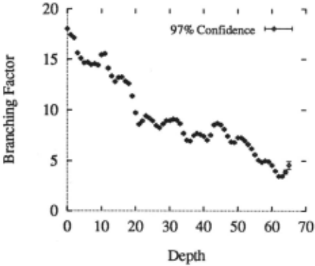
Figure 1 shows the results of 1000 samples with error bars representing the 97% confidence intervaL (Except for the rightmost points, the error bars are too small to distinguish in the figure.) The branching factor is time-dependent, where the number of enabled groups decreases through the night . The primary reason for a decreasing branching factor is that as groups are se­ lected for execution, the number of unscheduled groups decreases. Leaf nodes occur at approximately the same depth for a couple of reasons. First, the estimated du­ ration of all schedules is about the same. Second, the group durations in this particular scheduling problem do not vary much. The 1000 samples had a mean depth of 62.6 and a standard deviation of 0.8. The size of the search space is estimated by the product of the average branching factors; this data suggests that the number of schedules in the search space is on the order of 10 61 .

3.2 Search Space Quality

A schedule produced should not only satisfy all hard con­ straints but, ideally, should also achieve an optimal ob­ jective function score. 2 Hence, it is not solely the size of the search space that determines the difficulty of finding a good schedule; the density of quality schedules is also important. The same sampling method used to estimate search space size and shape can also be used to charac­ terize schedule quality density. Evaluating the schedules generated via iterative sampling yields a frequency dis­ tribution of scores which estimates the expected density of each score obtainable in the search space. We refer to this statistical estimate as a quality density function, and it is the basis for our ESQ method.

In determining the quality density function, it is im­ portant, yet often non-trivial , to obtain an unbiased sam­ ple from the solution space; i.e. , to sample the possible schedules uniformly. If the tree has a constant branching factor at every (internal) node and if all paths have the same length (i.e., if the search tree is balanced n-ary), then iterative sampling produces an unbiased, uniform sample. However, constant branching is not a necessary condition for uniform sampling, and it can be weakened as follows . If, for every depth, all nodes at that depth have the same branching factor, then iterative sampling will be uniform (assuming equal-length paths). As can be seen in Figure 1, the branching factor changes from depth to depth; however, the minuscule 97% confidence intervals indicate that the branching factor is nearly con­ stant for nodes at the same depth. (And, as argued above, the paths have approximately the same length.)

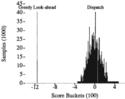
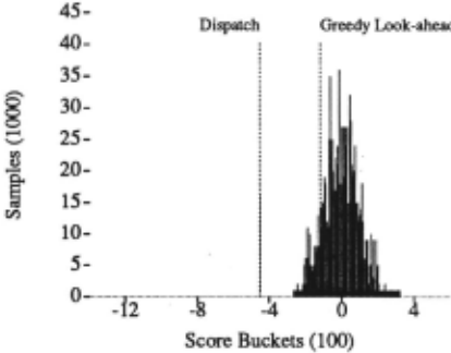
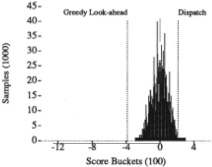
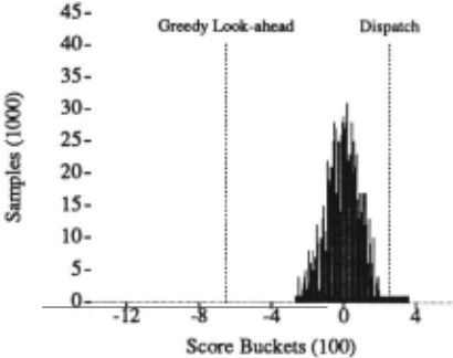
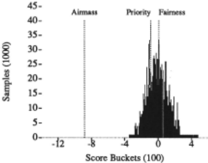
We performed 1000 iterative samples, and each sched­ ule generated was scored in terms of the composite ob­ jective function as well as in terms of each individual · attribute (priority, fairness, and airmass) . From these scores we constructed a quality density function for the composite objective and for each individual attribute. The resulting four density functions are shown in Fig­ ures 2-5. (The two dashed lines in each figure are discussed below.) The scores have been quantized into 100 "score buckets" of equal size. For each solid line, the x-coordinate is the mid-point of a score interval and the line's height indicates the number of samples that ob­ tained a score in that interval.

2 Another important consideration is schedule execution robustness; see [Drummond, Bresina, & Swanson, 1994].

3.3 Evaluating Scheduler Performance

We next describe how to evaluate scheduler performance using the quality density function, and we compare our two scheduling techniques with respect to quality den­ sity. In each of the four plots (Figures 2-5) , in addi­ tion to the quality density functions, we also indicate the performance of the two scheduling techniques. The single schedule generated by each technique was scored in terms of the composite objective function and in terms of each individual attribute. In each of the figures, the score obtained by a scheduler is shown by a dashed line (the height of the line is immaterial; it simply points to an x-axis value) . Note that the composite score (shown in Figure 2) obtained by each scheduler is the sum of the three attribute scores (shown in Figures 3, 4, and 5) .

As shown in Figure 2, greedy lookahead obtained a composite score of -11.56 and heuristic dispatch ob­ tained a composite score of +0.14. The difference be­ tween these scores is 11. 70; without knowledge of the dis­ tribution of scores, we do not know how significant this difference is. However, the quality density function en­ ables this difference to be interpreted more meaningfully. One such interpretation is in terms of the standard de­ viation from the mean. The quality density function for the composite scores (Figure 2) had an estimated mean of 0 and an estimated standard deviation of 1.30. Based on these estimated statistics, the lookahead score is 8.89 standard deviations better than the mean, while the dis­ patch score is 0.11 standard deviations worse than the mean. Interpreting the schedulers' performance against the background of the quality density function provides much more insight into just how much better greedy lookahead performed.

It is interesting that, with respect to the objective function, heuristic dispatch was no better than the mean value obtained by iterative (random) sampling. In contrast, the score obtained by greedy lookahead is better than all of the 1000 scores obtained by iterative sampling (Figure 2) . Notice that heuristic dispatch outperforms greedy lookahead with respect to the priority attribute (Figure 3). This is to be expected since group priority is the primary determinant of which group gets selected by the dispatcher, whereas, in the greedy search, priority has the same importance as the other two attributes.

When comparing scheduling techniques, in addition to schedule quality, it is also important to take into ac­ count the amount of time to generate a schedule. A nat­ ural performance measure that combines both of these scheduler performance factors is schedule quality divided by generation time. In order to make these two factors easier to combine, we can express schedule quality in units of time as well (hence, obtaining a unitless perfor­ mance measure). This can be accomplished by comput­ ing the expected amount of time for iterative sampling to generate a schedule that scores at least as well as a given schedule. Let p be the probability that a ran­ domly generated schedule scores at least as well as some given schedule. This probability is determined by the (cumulative) distribution function for schedule quality. 3 The expected number of iterative samples to generate such a schedule is then 1/p. Multiplying this expected number of samples by the computation time to perform one sample yields the expected sampling time measure of schedule quality. With this quality measure, a higher measure indicates better quality, and since lower sched­ ule generation time is preferred, a higher quality /time measure indicates superior performance.

This expected sampling time measure for schedule quality is based on more information about the quality density function than just its mean and standard de­ viation (i.e., it also takes into account the shape of the density function) . Hence, if the distribution function can be estimated accurately enough, this quality measure not only makes it easier to combine with generation time, but also yields a more discriminatory schedule quality com­ parison than the previously described metric of standard deviations from the mean.

3 The distribution function for schedule quality, F(x), equals J:O f(y) dy, where f(y) is the quality density function. Since smaller scores are better, the probability of randomly obtaining a score at least as good as xis equal to F(x).

We determined the schedule generation time for our two techniques, as well as for iterative sampling; this was done by averaging over 100 runs. The following are the results we obtained 4 : dispatch took 3.89 seconds, greedy lookahead took 98.75 seconds for ten iterations and iterative sampling took 3.76 seconds per sample. '

Assuming a normal distribution function, we can com­ pute the probability that a random sample will obtain a schedule score at least as good as some given score. This probability is 0.54 for +0.11 standard deviations and it is 3.06 x 10- 19 for -8.89 standard deviations.s' For the score obtained by dispatch, the expected number of samples is 1 / 0.54 or 1.85; and for the score obtained by lookahead, the expected number is 1 j 3.06 x 10- 19 or 3.27 x 10 18 . Multiplying by the time to perform one sam­ ple yields expected computation times of6.96 seconds for dispatch and 1.23 x 10 19 seconds for lookahead. For dis­ patch, the quality /time measure is 6.96 sees/ 3.89 sees or 1. 79; and for lookahead, it is 1.23 x 10 19 sees j 98.75 sees or 1.25 x 10 17 . Hence, greedy lookahead far outperformed heuristic dispatch on this problem; the ratio of the looka­ head measure to the dispatch measure is 7.0 x 10 16 .

In summary,· we started with the scores obtained by our two techniques, which had a difference of 11.70. This information told us that the lookahead scheduler achieved a better score, but there was no well-founded interpretation of how much better it was. Based on the results of statistical sampling, the quality /time measure yielded an interpretation of the lookahead score as being 16 orders of magnitude better than the dispatch score.

4 The results are CPU time for non-gc, user tasks from the Common Lisp time macro.

5 There may be some error between our sample distribu­ tion and the true distribution; furthermore, since the range of the objective function is bounded (within some unknown interval), the distribution is actually a truncated normal.

3.4 Search Heuristics

In traditional mathematical programming, the objective function is used to directly guide the construction of a solution. Certain assumptions are made about the form and behavior of the objective function that allow for the application of closed-form techniques to find optimal so­ lutions. AI approaches to constrained optimization typ­ ically assume that the objective function is so complex that closed-form solutions cannot be found. Typically, these approaches employ state-space search. For a par­ ticular problem instance (or class), heuristics are de­ signed that can help guide search toward a solution that scores well according to the objective function. How­ ever, it is often very difficult to design efficient search heuristics that effectively capture the information in the objective function. When the heuristic and the objective become too "decoupled", the heuristic can end up hav­ ing a different bias than that encoded in the objective and, hence, can fail to find high quality solutions.

One indicator of a bias discrepancy is when a signif­ icant portion of the quality density function is better than the heuristically selected solution's score. This is the case with the dispatch heuristic - its solution scored no better than the quality density function's mean value (Figure 2). Though this information indicates a bias discrepancy, it does not reveal the discrepancy's source, i.e., what information in the objective is not effectively encoded in the heuristic. This can be revealed by ex­ amining the heuristic's performance with respect to the individual objective function attributes. As seen in Fig­ ures 4 and 5, it is obvious that the dispatch heuristic is not taking into account fairness and airmass since its so­ lution scores worse, with respect to these two attributes, than almost all of the randomly found solutions.

After identifying some aspect of the objective function that is being ignored by the heuristic, one still has to de­ termine how to repair the heuristic. In general, this is a non-trivial problem; its difficulty depends on the com­ plexity of the objective function (i.e., how the attributes are combined) and on the form of the heuristic.

Since the solution found with the greedy heuristic scored better than all of the randomly generated solu­ tions, there is no obvious indication of a bias discrepancy - not surprising, since the greedy heuristic was identical to the objective function. However, we can still find such a discrepancy by looking at the quality density functions of the individual attributes. Recall that the objective function was designed to give equal importance to all three attributes. A solution which achieved a balanced tradeoff among the attributes should score equally well with respect to each attribute; that is, each attribute score of the solution should be the same number of stan­ dard deviations from the mean of the attribute's quality density function. However, as can be seen in Figures 3, 4, and 5, the solution found with the greedy heuristic does not score the same with respect to the attributes; rather it scores best on airmass, second best on priority, and worst on fairness. This imbalance can be corrected by adjusting the weighting factors on the attributes in the greedy search heuristic. Though the direction of the adjustment is obvious, finding appropriate weighting factors may take some experimentation (either manually or using machine learning techniques).

Though we used the objective function as a greedy search heuristic, this is not always best; e.g., the objec­ tive function may be too expensive to evaluate or some attributes may not be effective search heuristics (i.e. , an attribute's scores with respect to a partial solution may not be predictive of the scores of its completions) . The ESQ method can support the decision of which subset of the attributes to include in the search heuristic. Using the scheduler comparative analysis method illustrated in the previous section, we carried out the following em­ pirical evaluation. For each attribute, a greedy locka­ head search was performed using a heuristic based only on that single attribute (which is equivalent to zeroing the weights of the other two attributes in the compos­ ite search heuristic). For each single-attribute greedy search, the best schedule found was evaluated in terms of the (original) composite objective function.

Figure 6 shows the three composite scores obtained by each single-attribute search heuristic against the back­ ground of the same composite quality density function as in Figure 2. These results indicate that airmass is the best single-attribute local heuristic; i.e., partial sched­ ules that score well with respect to airmass are likely to be prefixes of complete schedules that score well with respect to the composite objective function. The re­ sults also indicate that fairness is the worst local pre­ dictor, which makes sense since it is the "most global" attribute in the objective function. That is, there are schedules that, while rated highly (perhaps even opti­ mally) with respect to fairness, have prefixes that score poorly. For example, consider a schedule that assigns each user's groups fairly, but gives each user a contigu­ ous interval of time. While the final schedule scores well , its prefixes score poorly, and would not be found during search. The fairness heuristic prefers schedules that fre­ quently alternate between users. Priority turned out not to be a very good local heuristic either, which explains why ATIS dispatch did not perform well with respect to the composite objective function.

4 General Application of ESQ

In this section we discuss how the ESQ method can be applied in more general contexts. Our ESQ character­ ization was done under the assumption that iterative sampling in the search tree produces a uniform sample from the space of possible solutions. Our formulation of the scheduling problem has two beneficial characteris­ tics that make it easy to satisfy this assumption. Firstly, nodes at the same depth in the search tree have nearly the same branching factor and the lengths of paths are approximately the same length. Because of this, sam­ pling uniformly at each branch point implies that the leaf nodes are uniformly sampled. Secondly, the search tree includes only feasible schedules, i.e., schedules that satisfy all the hard constraints. Hence, uniformly sam­ pling the search tree leaf nodes implies a uniform sam­ pling of the solution space. In our case, the search tree is chronologically organized; however, as long as there is a one-to-one correspondence with leaf nodes and solutions, then the ESQ method as described directly applies.

Due to the shape of the search tree for our telescope scheduling problem, it was easy to uniformly sample the leaf nodes; however, in general, this is not trivial. To guarantee uniform sampling of the leaf nodes, the ran­ dom selection at each branch point must be biased by the size of the subtree below each choice. That is, the prob­ ability of selecting a particular child node must be equal to the proportion ofleaf nodes in the child's subtree (rel­ ative to the total in the current node's subtree). Within the field of randomized algorithms, theoretical and prac­ tical results have been obtained for randomized approx­ imate counting and almost uniform generation of com­ binatorial structures; for example, see [Sinclair, 1993; Jerum, Valiant, & Vazirani, 1986]. These results can help in the construction of algorithms that almost (i .e., with small bias) uniformly sample a tree's leaf nodes.

There is another potential problem with general appli­ cation of the ESQ method. In many search formulations, not all leaf nodes correspond to solutions- some are fail­ ure nodes. These failures are incorporated into the ESQ method as follows. As before, the leaf nodes are uni­ formly sampled; however, the quality density function for solutions is computed based only on the non-failure leaf nodes. The probability offailure, P!, is estimated by the number of failure leaf nodes encountered during the sampling divided by the number of samples. As before, we compute the probability, Pb, that a randomly gener­ ated schedule would score at least as well as some given schedule. The probability, p, that a random sample pro­ duces a sched,ule that scores at least as well as some given schedule is then the product Pb · (1- P! ). Using p, the quality /time measure is computed as before.

In our telescope domain, we have all day to schedule; hence, whenever the scheduling problem changes (due to modified or new observation requests), we can afford to carry out a new set of ESQ experiments in order to re­ tune our search heuristics. However, in other domains, this may not be feasible. In such cases, it may be possible to select a representative suite of problem instances and base the ESQ statistical evaluation and search heuristic tuning on the combined samples of these problems.

5 Summary and Conclusion

This paper's main contributions are the ESQ method for characterizing scheduling problems and evaluating scheduler performance and the demonstration of this method in a practical telescope scheduling domain. We demonstrated how the ESQ method can provide an es­ timate of the size and shape of the search tree and can provide a quality /time measure of scheduler per­ formance. In addition, we illustrated how the method can support the construction of more effective search heuristics. While we have been concerned with schedul­ ing techniques and scheduling problems, the ESQ method should apply more generally within the larger class of constrained optimization problems.

The ESQ method is statistical, employing a Monte Carlo algorithm called iterative sampling. In summary, the complete ESQ method involves the following steps:

1. Based on the shape and size of the search tree, uni­ formly sample the tree; from this sample, compute the frequency distribution of schedule quality and the failure probability, P!.
2. From the frequency distribution, characterize the quality density function . That is, compute the sam­ ple mean and standard deviation of the schedule scores, and determine the distribution type. (In the example presented, the distribution was normal.)
3. Express the scheduler's score in terms of standard deviations from the quality density function's mean.
4. Using the distribution function, determine the prob­ ability, Pb, that a randomly generated schedule will score at least as good as the scheduler's score. Then compute the probability, p, that a random sample will produce such a schedule as Pb · (1- P! ) .
5. Compute the expected time for iterative sampling to obtain a score at least as good as the given score by multiplying the expected number of samples re­ quired, 1/p, by the time to perform one sample.
6. Compute the quality /time measure as the expected iterative sampling time (computed in previous step) divided by the scheduler's computation time.

In some sense, our quality /time measure is a "com­ mon currency" for expressing scheduler performance on a given problem. In addition to comparing the perfor­ mance of different schedulers, the ESQ method can also be employed for the following purposes: ( i) to compare the difficulty of different problems with respect to a given scheduler; ( ii) to evaluate the impact of different search formulations with respect to scheduler performance; (iii) to evaluate the impact of different objective functions with respect to problem difficulty for a given scheduler.

Recall that our nondeterministic greedy lookahead chose the best schedule after ten iterations; this number of iterations was chosen arbitrarily. With more itera­ tions, the algorithm might find a better schedule - al­ though at a higher computational cost . Using our qual­ ity /time measure, we could empirically determine the number of iterations that yields the most cost-effective performance. This type of algorithm tuning could be applied to any scheduler whose performance behavior varies depending on the amount of computation time al­ located. Similarly, we could empirically determine the amount of lookahead that is most cost-effective (recall that our greedy algorithm used one-step lookahead). We intend to carry out such experiments in the future.

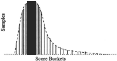
In addition to the reported uses of the quality den­ sity function, we speculate that (in some cases) it can be useful in characterizing the difficulty of a problem. For example, consider the hypothetical quality density func­ tion in Figure 7. One might conclude that this problem is intrinsically easy since there are so many high quality solutions and not many low quality ones. Even an unin­ formed search (like iterative sampling) can quickly find a high quality solution for such a problem. In cases that are not so extreme, it is less obvious how to relate shape of quality density and problem difficulty. This topic re­ quires further research.

The experiments reported in this paper used a Lisp­ based scheduling engine. However, in order to make the system useful to astronomers, we have had to re­ implement it in C so that they themselves can extend and support it. This new system will provide a self eval­ uation facility which will automatically perform the ESQ characterization experiments upon request. The final version of the system will be accessible to users via the Internet and will accept new ATIS groups on a daily ba­ sis. Thus, the definition of the scheduling problem will change frequently. We expect that a telescope manager will be able to use the self evaluation facility to track the changing characterization of the search space. Based on the current characterization, a telescope manager could choose the best scheduling method and search heuristic for the current mix of ATIS groups. It would be useful if the system itself were able to make these choices. Work along these lines is reported by Greenwald and Dean (1994), where Monte Carlo simulation builds a picture of the search space that can be used to detect and 1 avoid potential schedule bottlenecks. Exploring the use of ESQ in this context is a topic for future work.

Acknowledgments

We would like to thank Will Edgington and Ellen Drascher for their significant contributions towards mak­ ing the automatic telescope software a reality. For their helpful feedback on this paper, we would like to thank Lise Getoor, Rich Levinson, Steve Minton, Nicola Muscettola, and Barney Pell.