Logic Programming for Robot Control

1 Introduction

Since Shakey and STRIPS [Fikes and Nilsson, 1971], logic and robotics have had a tumultuous history together. While there is still much interest in the use of logic for high-level robotics (e.g., [Les¢rance et al., 1994; Caines and Wang, 1995]), there seems to be an assumption that low-level 'reac­ tive' control is inherently alogical. This paper challenges this assumption.

This paper investigates the idea of using logic programs as a representation for the control of autonomous robots. This should be seen as logic programming in the sense of logic + control [Kowalski, 1979]; we use a logic program to specify what to do at each time, and use an execution mechanism that exploits a derived notion of 'state' in order to make it practical.

The main highlights of this approach are:

1. An agent can be seen as a transduction: a function from inputs (sensor values) into outputs (action attempts or

*Scholar, Canadian Institute for Advanced Research

actuator settings). These are 'causal' in the sense that the output can only depend on current inputs and previous inputs and outputs. This function will be represented as a logic program specifying how the output at any time is implied by current and previous inputs. The causality ensures that we have acyclic rules.

1. The logic programs are axiomatised in phase space [Dean and Wellman, 1991] (the product of space and time, i.e., the predicates refer to times as part of the axiomatisation) in a similar manner to the event cal­ culus [Kowalski and Sergot, 1986]. This allows us to axiomatise persistence as well as accumulation (integra­ tion) over time and differentiation with respect to time.
2. The notion of 'state' is a derived concept; the state is what needs to be remembered about the past in order for the agent to operate in the present. The axiomatisation is in terms of how the 'current' action depends on cur­ rent inputs and past inputs and other values; the state is derived so that the output, instead of being a function of the current inputs and all past history, is a function of the current inputs and the state.
3. Although the specification of what to do looks like a Prolog program, it is not evaluated as a Prolog program. Instead we exploit the fact that the agent exists in time; that inputs are received in sequence, and that all previous inputs have already been received (and no subsequent inputs have been received) when the agent makes a de­ cision. Instead of treating this as a logic program that may need to do arbitrary computation reasoning about the past, we actively maintain a state. The reasoning about what to do at any time depends only on the current inputs and the remembered state.

This perspective is useful for a number of reasons:

1. It provides for a representation for an agent's behaviour in a language with a well defined semantics (see [Apt and Bezem, 1991]).
2. It lets us model both the robot and the environment within the same language. The robot axioms can be evaluated in two modes. In the 'situated' mode, the agent gets sensor values directly from the environment, and acts in the environment. In simulation mode, we also have a model of the environment, and can run the models together as a simulation of the integrated system.

1. There is a clean way to integrate this with models of uncertainty (e.g., for noisy sensors and sloppy and un­ reliable actuators). The logic programs here are of the fonn that can be used within a probabilistic Hom abduc­ tion system (Poole, 1993]. One of the aims of this work is to produce a representation for robot behaviour that is both suitable for controlling a real robot and also can be the output of a decision-theoretic planning system.
2. The logic programs form an executable specification of what an agent should do. Although they can be evalu­ ated reasonably quickly using current logic programming technology, it may be possible to compile these speci­ fications into circuits for robots (in a manner similar to [Gaboury, 1990]).
3. It shows how two traditions in AI (namely logic-based AI and robot programming), seemingly at odds, can be unified. Whether we are successful in this remains to be seen. In particular, this paper should be seen as a proposal and an initial feasibility study- there is still much work that remains to be done before this is a competitor for programming robots.
4. Inspired by constraint nets [Zhang and Mackworth, 1995], this work shows how to model hybrid continuous­ discrete systems. The axioms will all be true (in the limit) for continuous time. We derive discrete events from con­ tinuous time.

2 Representation

The problem that we are trying to solve is to represent, simu­ late and build an agent that senses and acts in the world. The agent receives a sequence (trace) of inputs (percepts or sensor values) and outputs a sequence (trace) of outputs (actions or actuator settings).

We assume a time structure T that is totally ordered and has a metric over intervals. T can either be continuous or discrete. A trace is a function from T into some domain A.

A transduction is a function from (input) traces into (out­ put) traces that is 'causal' in the sense that the output at time t can only depend in inputs at times t' where t' :5; t. An agent will be a specification of a transduction.

Transductions fonn a general abstraction of dynamic sys­ tems [Zhang, 1994; Zhang and Mackworth, 1995; Rosen­ schein and Kaelbling, 1995]. The problem that we consider is to use logic programs to specify transductions.

The language that we use is that of acyclic logic programs [Apt and Bezem, 1991 ], with a limited repertoire of predicates that explicitly refer to time. We assume that the acyclicity corresponds to temporal ordering (if time t 1 is before time t2 then predicates referring to time t1 will be lower in the acyclic indexing that those referring to time t2). We will use negation as failure - for those who do not like this, we mean the completion of the program (which forms a sound and complete semantics for acyclic programs [Apt and Bezem, 1991]). The axioms below assume a limited fonn of arithmetic constraints.

A fluent [McCarthy and Hayes, 1969] is a function that depends on time. Each fluent has an associated set called the range of the fluent. A propositional fluent is a fluent with range { true,false} . Syntactically a fluent it a tenn in our language.

Definition 2.1 An agent specification module is a tuple (I, 0, R, L, A} where

• I is a set of fluents called the inputs. The inputs specify what sensor values will be available at various times. The range the the input trace is the cross product of the ranges of the fluents in the inputs. Atom sense(Fl, Val, T) is true if input fluent Fl has value Val at timeT.
• 0 is a set of fluents called the outputs. An output is a propo­ sitional fluent that specifies actuator settings at various times. These can also be seen as the actions of the agent (in particular, action attempts). The atom do( F l, Val, T) is true if the agent sets actuator Fl to value Val at time T, or to 'do' action Fl = Val at timeT.
• R is a set of fluents called the recallable fluents. These are fluents whose previous value can be recalled. Recallable fluents will be used to model persistence as well as inte­ gration and differentiation.
• L is a set offluents called the local fluents. These are fluents that are neither inputs, outputs nor recallable. The pred­ icate val(Fl, Val, T) is true iflocal fluent Fl has value Val at timeT.
• A is an acyclic logic program. A specifies how the outputs are implied by the inputs, and perhaps previous values of the recallable fluents, using local fluents, arithmetic constraints and other (non-temporal) relations as inter­ mediaries.

The interface of agent specification module (I, 0, R, L, A} is the pair (I, 0}.

Each rule in the logic program has a 'current' time, to which the predicates refer. There are a restricted facilities for referring the past (i.e., to values of fluents in 'previous' times). In particular, an agent cannot recall what it hasn't remembered. There is one facility for specifying what needs to be remembered, and two predicates for recalling a value (these provide the predicates for use with recallable fluents):

• set( F l, Val, T) is a user-defined predicate that specifies that recallable fluent F I has value Val at time T. Only fluents that are specified in this way can be referred to in the future.
• was(Fl, Val,T1,T) is a predicate that specifies that re­ callable fluent Fl was assigned value Val at time T1 and this was the latest time it was given a value before time T (so Fl had value Val immediately before time T). It is axiomatised in a manner similar to the event calculus [Kowalski and Sergot, 1986] (see Section 4.5):

was(Fl, Val,T~tT)­

time(Tl) I\

T, <TI\

set(Fl, Val, Tl) I\

,...., reset.before(Fl, T~o T).

where reset.before(Fl, T~o T) is true if fluent Fl was assigned a value in the interval (T" T):

reset.before(Fl, T~o T) -

time(T2)

T,<T21\

T2<TI\

set(Fl, V2,T2) .

The predicate time(T) is defined in Section 2.4, where we consider the problem of representing dense time.

• now(Fl, Val, T) is a predicate that specifies that recallable fluent F 1 has value Val at time T. It can be axiomatised as follows:

In user programs, the following restrictions apply:

• set cannot appear in the body of any (user) clause. It only appears in the body of the rules given above. It does however appear in the head of user clauses.
• now or was (or reset or reset..before) do not appear in the head of any user clause. They are defined by the clauses above.
• All times referred to in clauses must be to the same time (the 'current time' of the clause), with the exception of the third parameter of was, and the predicate now can refer to times before the current time of the clause 1 , and arithmetic comparisons can be used on times.

2.1 Pure Reaction

We can model pure reaction, that is memory less systems built from combinational networks (as in, e.g., [Agre and Chapman, 1987]), where the output is a function of the immediately available inputs. A logic program (with all fluents referring to the same time) can represent arbitrary combinatorial circuits.

2.2 Persistence

The use of set, now and was allows recallable fluents to persist. Once a value of a fluent is set that value persists until a new value is set. At any time it is always the last value set that we look at (it is this property that allows us to build efficient implementations)-where 'last' means means 'before now' for was and 'at or before now' for now.

When setting the value of fluent.fl at time T, we cannot use now for that fluent and time in the proof for set, as this violates the acyclicity assumption. We can however, use the was predicate for that fluent and time.

Persistent values are true in left closed, right open intervals. If fluent fl was set to value v at time t 1 and was set to a different value at time t2 (and no other settings for value v occurred in between), then the fluent fl has value v in the interval [t1, t2). This is the opposite convention to the event calculus [Shanahan, 1990]. We want this convention as robots have internal state so that it can affect what they will do; if a robot realises at time t2 that it should be doing something different, then it should change what it is doing immediately, and not wait.

This notion of persistence is close to that of the event calcu­ lus [Kowalski and Sergot, 1986; Shanahan, 1990] (see Section 4.5).

1 This is to allow us to model 'transport delays' (see Section 4.2), that are essential for the modelling of analogue systems. In general using this facility means that we have to maintain a history of set values and not just a state of set values.

2.3 Integration and Differentiation

One of the reasons for axiomatising in phase space and making time explicit is that we can integrate over time. We will assume that anything we try to integrate is Riemann integrable.

If we want to produce the value of some accumulative predicate, we can use

where f ( t) = d~~ t) · For any fixed 6 we can compute the sum recursively. The integral is the limit as 6 approaches zero. We can write the sum that approaches the integral using the following schema (with a rule for each integrable fluent fl):

Similarly we can axiomatise the derivative of a fluent with respect to time using the schema for each differentiable fluent ft! .

Solving these may involve some constraint solving.

Before we define 'true in the limit', we discuss some issues relevant to the acyclicity restriction. Suppose, the derivative of integrable fluentfl is a function of the value offl atT (e.g., the force of a spring is a function of the position of the object). To define the clause for the derivative, we need to determine the value of fl at time T, but cannot have now(fl, V, T) in the body of a rule to prove val( deriv(fl), DJ, T), as this violates the acyclicity constraint. There are two solutions to this problem: the forward Euler and the backward Euler.

Assume the relation val(deriv(fl, V),DF,T) is defined which means that DF is the derivative of fl at timeT, with V being fl's value.

The 'forward Euler' uses the 'previous' value of V (i.e, the value Vt in the integration clause above). This is correct as 'in the limit' V = Vt .

This solution turns out to have problems with the stability of discretizations. The 'backward Euler', which works better in practice, uses the 'future' value for the derivative:

2 These rules are schemata as we have to choose whether a fluent is integrable or derivable (or neither). A fluent cannot be both: we cannot use the differences in values to compute derivatives as well as using derivatives to compute differences in values. This violates the acyclicity restriction, and leads to infinite regress.

Solving this may involve some constraint solving.

2.4 Truth in the limit

The axioms given for was and now are incomplete - they do not specify the structure of time.

If time is discrete 3 , then there are no interpretation problems with the axioms above. In particular, we make the predicate time(ta) true for each 'time' t,. The predicate was always refers to the previous time point (or to the last time point when the value was set), and there is always some finite duration of each time interval.

If time is continuous, there are semantic difficulties in in­ terpreting these sentences (in particular the integration and differentiation formulae that allow for the setting of values at each time point). We cannot interpret the integration and dif­ ferentiation axioms 'in the limit', as in the limit, V = Vi and T = T1; the integration axioms become cyclic (and tautolo­ gies), and the differentiation axioms provide no constraints on the value of D f.

In order to be able to interpret the above sentences we have to consider the limit as finite discretizations become finer and finer (in the same way that integration is defined). The axioms will talk about what is true for each discretization. The values that 'was' refers to will be well defined for each of these discretizations. The meaning for the continuous case will be what is true in the limit.

To define the limit, consider a uniform discretization with time interval dt > 0. For each dt we consider the discretiza­ tion that consists of the time points k x dt for some integer k.

Definition 2.2 Axioms A entails fluent f has value v under discretization dt > 0 at timet, written A Fdt now(!, v, t) if

where F= denotes truth under Clark's completion, or in the (unique) stable model, or one of the other equivalent semantics for acyclic logic programs [Apt and Bezem, 1991], of the axioms together with axioms defining arithmetic.

Definition 2.3 Axioms A entails fluent f has value v in the Hmit at time t, written A Foo now(!, v, t), if for every f > 0 there exists 6 > 0 such that if 0 < dt < 6, then A Fdt now(!, v', t) where lv- v'l < f.

One subtlety should be noted here. We can ask about now(!, v, t) for any t even if time(t) is not true- if this were not the case these definitions would not work, as most values of dt 'miss' any particular time (i.e., for most times t and increments dt there does not exist and integer k such that t = k x dt). Being an official 'time' only constrains what past values can be referred to.

Note that we never consider the theory with the infinite partition.

3 By discrete I mean that there are no sequences of different values which get closer and closer (Cauchy sequences - see e.g., [Zhang and Mackworth, 1995]). Informally this means that there are only finitely many time points between any two time points.

3 An Example in Detail

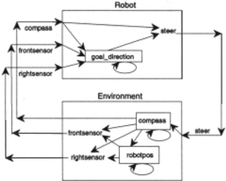
We demonstrate the representation using an example of mod­ elling a robot and an environment. These two axiomatisations will highlight different features; the robot model will highlight reactive systems with remembered events; the environment model will highlight integration over time.

The example is of a maze travelling robot that is continu­ ously trying to go East (i.e., at 0° orientation), but may have to avoid obstacles. The robot can sense obstacles and its di­ rection of travel, but only has control over its direction of steering.

3.1 Robot Model

We assume that the robot can sense which direction it is trav­ elling in, has a sensor on the front of the robot and a sensor on the right that can detect obstacles. The only control that the agent has is to change the steering angle - we assume that the agent can instantaneously change from steering left, right or straight (but steering takes time to achieve the desired effect). This example is adapted from [Zhang, 1994].

For the robot specification, we axiomatise what the steering should be depending on current, and perhaps previous sensor values.

We use the following predicates defining the inputs at dif­ ferent times:

sense( compass, C, T) means that the robot is sensing that it is heading in direction C at time T. All directions are in degrees anticlockwise from East (i.e., the standard directions in an x-y graph). ·

sense(lront, blocked, T) means that the front sensor is de­ tecting an obstacle at time T.

sense( right , blocked, T) means that the right sensor is on at timeT.

and the output:

do( steer, D, T) means the robot should steer D-wards at timeT where D E {left, right, straight}.

The following clauses axiomatise a 'bang-bang' controller that specifies which direction to steer based on the compass reading and the current desired direction of the robot. In these clauses, now(goaLdirection, G, T) is true if the robot wants to go in direction G at time T:

do(steer,left,T) +­ now(goaLdirection, G, T) 1\ sense( compass, C, T) 1\ (G- C + 540) mod 360- 180 > 5. do( steer, straight, T) +­ now(goaLdirection, G, T) 1\ sense( compass, C, T) 1\ I(G- C + 540) mod 360- 1801 :55. do( steer, right, T) +­ now(goaLdirection, G, T) 1\ sense( compass, C, T) 1\ (G- C + 540) mod 360- 180 < -5.

5° is an arbitrarily chosen threshold.

The goal direction depends on current and previous sensor values. The robot changes the goal direction when it is trav­ elling in the previous desired direction 4 and it finds its way blocked, in which case it now wants to travel at goo to the left of where it was travelling:

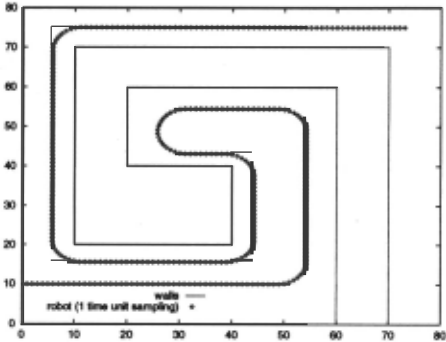
set(goal...direction, D +go, T) +­ sense( compass, C, T) 1\ was(goaLdirection, D, _, T) 1\ same(C,D) 1\ sense(front, blocked, T).

Alternatively the robot changes its desired direction by goo to the right if it is travelling in the previous desired direction, it is not blocked on the right and is not going in its ultimate desired direction (which is 0°). Note that sometimes the desired direction is 360° - in this case it still wants to tum right to follow the right wall - this will enable the robot to get out of maze traps (such as the maze in Figure 2).

set(goal...direction, D - go, T) +­ sense(compass,C,T) 1\ was(goaLdirection, D, _, T) 1\ same(C,D) 1\ D ::/; 01\ '""' sense (front, blocked, T) 1\ '""'sense( right, blocked, T).

In order to allow for noise and sampling error the robot needs only the desired direction to be within some margin of error to the current direction. The predicate same(Dt. D2) is true if directions D1 and D2 are the same up to this error.

With this model, we can derive what to do at any time based on what sensor values it has received.

4 This means that the robot designer (and modeller) does not need to consider how the sensors work in the middle of a tum. This was chosen to show how 'events' can be derived from continuous change.

Such a logic program could be run as a situated robot that gets sensor values from the environment and acts in the envi­ ronment (see Section 3.3). In this paper, in order to (a) show the generality of the model, and (b) to show how integration over time can work, we will use the same language to model the environment. The environment model together with the agent model can be used to simulate the system.

3.2 Environment Model

We assume that the environment is another agent like the robot. It bas inputs (from the output of the robot) and has out­ puts which can be sensed by the robot. The two models can be joined together to form a feedback control system. The main constraint is that the conjoined logic programs are acyclic [Apt and Bezem, 1gg1] with the indexing due to acyclicity constrained to be temporal.

Whether the front sensor is on depends on the position of the robot, the direction of the robot and whether there is a wall close to the robot in front of the robot. Here robotpos(X, Y, T) means that the robot is at position (X, Y) at time T. seeblock(X, Y, D) is true if the robot can detect a wall in direction D from position (X, Y)- this does not depend on the time, but only on the position and direction of the robot.

Similarly we can axiomatise sense( right, blocked, T), and sense( compass, D, T) and can axiomatise the maze using seeblock.

The position of the robot is the integral of the velocities overtime:

set( compass, (C +CD x (T- T1) + 360) mod360,T) +- was( compass, C, T1, T) 1\ val(deriv(compass), CD,T1).

The derivatives are axiomatised as follows: If robot is steering left, DC I DT = 10 (i.e., 10 degrees per time unit). If robot is steering straight, DC I DT = 0. If robot is steering right, DC I DT = -10.

val(deriv(compass), 10,T) +­ do( steer, left, T). val(deriv(compass),O,T) +­ do( steer, straight, T). val(deriv(compass), -10, T) +­ do( steer, right, T).

The position of the robot is the integral of velocities:

The following axioms define the x derivatives and the y derivatives of the position with respect to time. We are as­ suming that the speed is 1 and that cos and sin use degrees (as opposed to, say, radians),

3.3 Computation

If we were to run the above axiomatisation as a Prolog pro­ gram, the code is hopelessly inefficient The problem is that we have to consider all previous times to check whether an event occurred (at least all previous times where inputs ar­ rived). Moreover to check whether an event occurred, we have to check all previous times to check whether a previous event occurred. As you can imagine, such computation is hopelessly slow.

In order to make this efficient, we take advantage of the fact that we are evaluating in time: at each time all previous observations have arrived and no subsequent observations have arrived. We exploit the fact that all of the references to the past are in terms of of was. Instead of using the axioms defining was explicitly, we actively maintain a state, always remembering the latest values that were set. The predicate was can be implemented by looking up the lastest set values. In other words, the set values are remembered forming the state of the agent. The logic program is evaluated by proving the output from the current inputs and the current state.

Figure 2 shows a simulation of the robot in the maze. It is simulated by discretising time with one time unit intervals. Other discretizations, as long as they are not too coarse give similar results.

The above simulation (of both the robot and the environ­ ment), ran faster than 20 steps per second, on a 68040 running Sicstus Prolog. · Partial evaluation should be able to speed this up, and it seems that it should be possible to compile the logic program specification into hardware (as does [Gaboury, 1990]). Thus it seems as though the logical specification of robot action is not impractical from an efficiency point of view.

4 Discussion and Comparison

This paper is not intended to just define yet another robot programming language. Let us take the very general view of an agent as a 'causal' function from input history to outputs

[Zhang and Mackworth, 1995; Rosenschein and Kaelbling, 1995]. Suppose we want to use logic as a formal specification for the actions of the robot, for example in order to prove theorems about the robot behaviour. If we are to treat values of the inputs at various times and values of the outputs at various times as propositions, then the constraint imposed by the robot function is that it can't be the case that the inputs have certain values and the output is not the appropriate function of the inputs; but this is exactly the definition of a definite clause: inputs imply the outputs.

It might be argued that the logic here is too weak to represent what we want to, for example it cannot represent disjunction. We have to be careful here; if a robot is to do something, it cannot be unsure about its own actions. It must commit to one action in order to carry it out A robot cannot 'do' action a1 V a2 without doing one of them. This does not mean that the agent cannot be ignorant (or unsure) of what other agents will do, or be unsure about what values it will receive from the environment. For a general discussion of these issues, and a way to handle them within the logic presented here (by allowing independent 'choices' made by different agents and nature) see [Poole, 1995].

4.1 Noisy sensors and actuators

The above axiomatisation showed how to model partial in­ formation about the environment (the agent had very lim­ ited sensing ability). In this section we sketch a way to model noisy sensors and actuators using a continu­ ous version of probabilistic Horn abduction [Poole, 1993; 19951.

The general idea of probabilistic Horn abduction is that there is a probability distribution over possible world gen­ erated by unconditionally independent random variables. A logic program gives the consequences of the random choices for each world. Formally, a possible world selects one value from each alternative (disjoint set); what is true in the possible world is defined by the unique stable model of the selection and the acyclic logic program [Poole, 1995]. The probability of the world is the product of the probabilities of the values selected by the world. In this framework, the logic programs can still be interpreted logically, and the resulting framework, although based on independent random variables, can repre­ sent any probability distribution [Poole, 19931.

To model noisy sensors, we add an extra 'noise' term to the rules. For example, to represent additive Gaussian noise for the compass sensor, with standard deviation 3, we can use the rule:

Where for all T, {val( c..noise, N, T) : -N E ~}is an alterna­ tive set. val ( c..noise, N, T) is true in world w if the compass noise is N standard deviations from the mean at time T in world w (each world has a unique N that is true for each time). N is normally distributed with mean 0 and standard deviation 1 (this is usually called the z-score):

With such a noisy sensor the agent could do dead reckoning; maintaining its own record of its position. However if the actuator is also unreliable, then the errors explode. Unreliable actuators can be modelled similarly to the noisy sensors, for example,

Where a_error is treated analogously to c_noise.

When the dynamics are linear and the noise is Gaussian, the posterior distributions can be solved analytically, as in the Kalman filter (see [Dean and Wellman, 1991]).

4.2 Constraint Nets

Constraint nets [Zhang and Mackworth, 1995] form a mod­ elling language for hybrid systems that combines discrete and continuous time, and discrete and continuous domains into a coherent framework. This is done by abstracting the notion of time so that it covers both discrete and continuous models of time, and using 'events' as the interface between continuous and discrete time.

Constraint nets are built from three basic transductions~ Transliterations, which do not depend on the past, are axioma­ tised here by allowing (acyclic) logic programs to specify how current outputs depend on current inputs. Our was predicate corresponds to unit delays. Transport delays of time r can be modelled as the atom now( Fl, V, T - r) -to implement these we have to maintain a history of at least r long, and not just a state.

4.3 Logic Control

COCOLOG [Caines and Wang, 1995] is a logic for discrete control that shares many features of the discrete form of the logic here. The main difference is that in COCO LOG, the state of the system is an explicit term of the language. The language is also more complicated than the simple Horn clauses used here and the main control loop is extra-logical.

The declarative control of Nerode and Kohn [1994] uses Prolog for control. Their main aim is for a Prolog program to prove that some action is optimal. Their Prolog rules are at a much different level than the simple rules used here, which are impractical when using Prolog's back-chaining search strat­ egy.

4.4 GOLOG

GO LOG [Les¢rance et al., 1994] is a programming language for robots based on the situation calculus. Unlike the proposal in this paper, GOLOG programs are not sentences in a logic. Rather the logic is at the meta-level providing a semantics for the Algol-like GOLOG language.

One intriguing idea is to use the logic programming ap­ proach here to write a low-level controller that interprets GOLOG programs. This could be done by having two state variables, one that is the current action the agent is 'doing' and one is a list of actions 'to do'. The rules could be used to reduce expressions in time, for example to interpret action sequences we can use:

Similarly, we can interpret more complicated constructs such as while loops as well as monitoring 'primitive' actions (e.g., we can see setting the goal direction in the above example as a high level action that decomposes into continuous action, and is monitored as to when it is complete). A full discussion of this is beyond the scope of this paper.

4.5 Event Calculus

The event calculus [Kowalski and Sergot, 1986; Shanahan, 1990] provides a mechanism to represent persistent proper­ ties over intervals from events that make the properties true and false. What is new in this paper is deriving events from changes in continuous properties, having cumulative proper­ ties, and exploiting evaluation in time to gain efficiency.

There is quite a simple translation to map the event calculus irito the framework of this paper. The event calculus uses the predicates: happens( E, T) is true if event E happens at time T; initiates(E, P) is true if event E makes P true; terminates(E, P) is true if event E makes P no longer true. These can be mapped into the fluent representation used here:

If we want the convention used in this paper that predicates are true in left closed intervals, we can represent holds( P, T), (meaning predicate P holds at time T) by:

One main advantage of our representation is that, when we act in time, and all of the set's are done in temporal ordering, and we maintain a state, then we can implement holds very fast, by looking up the last value that was assigned to the variable.

Shanahan's notion of 'autotermination' is similar to our deriving events from continuous change.

4.6 Other Mixes of Logic and Continuous Time

There have been other proposed mixes of logic and continu­ ous time (e.g., [Sandewall, 1989; Shanahan, 1990; Dean and Siegle, 1990; Trudel, 1991; Pinto and Reiter, 1995]), but in all of these either "during the time span of a situation no ftuents change truth values" [Pinto and Reiter, 1995] or the axioma­ tiser needs to know a priori how properties accumulate (they effectively do integration off-line). For robot control, we do not know how the sensor values will change; the best we can do is to derive (estimate) integrals online. None of these other proposals let us do this.

5 Conclusion

This paper has argued the logic programs can be used effec­ tively as a programming language for robot control. The logic program forms an executable specification of what the robot should do. The same language can be used for modelling the robot and the environment (and also multiple robots). This axiomatisation can be combined with probabilistic Hom ab­ duction [Poole, 1993] to allow for modelling uncertainty in the environment (e.g., exogenous events, noisy sensors and unreliable actuators).

This paper has not described some ideas about improving efficiency by adaptive sampling: by partially evaluating the logic program, we can determine what inputs we must look for in order for an event to occur. When running the robot, we can build into our sensors detectors for these conditions; when detected, we can run the program in a forward direction to derive events. In the simulation, we can query the envi­ ronment to determine when these events would occur. Such ideas are currently being pursued.

Acknowledgements

Thanks to Alan Mackworth and Ymg Zhang for interesting discussions on hybrid systems. Thanks to Mike Horsch for comments on a previous draft. This work was supported by Institute for Robotics and Intelligent Systems, Project IC-7 and Natural Sciences and Engineering Research Council of Canada Operating Grant OGP0044121.