
Learning One More Thing
Proceedings of the Fourteenth International Joint Conference on Artificial Intelligence. Learning. Pages 1217-1224.
© 1995 International Joint Conferences on Artificial Intelligence
Abstract
Most research on machine learning has focused on scenarios in which a learner faces a single, isolated learning task. The lifelong learning framework assumes that the learner encounters a multitude of related learning tasks over its lifetime, providing the opportunity for the transfer of knowledge among these. This paper studies lifelong learning in the context of binary classification. It presents the invariance approach, in which knowledge is transferred via a learned model of the invariances of the domain. Results on learning to recognize objects from color images demonstrate superior generalization capabilities if invariances are learned and used to bias subsequent learning.
- [Baxter, 1995] J. Baxter. The canonical metric for vector quantiza- tion. submitted for publication, 1995.
- [Caruana, 1993] R. Caruana. Multi task learning: A knowledge- based of source of inductive bias. In Paul E. Utgoff, editor, Proceedings of the Tenth International Conference on Machine Learning, pages41-48, San Mateo, CA, 1993.
- Morgan Kaufmann. [Hild and Waibel, 1993]
- H. Hild and A. Waibel. Multi- speaker/speaker-independent architectures for the multi-state time delay neural network. In Proceedings of the International Confer- ence on Acoustics, Speech and Signal Processing, pages II 255- 258. IEEE, April 1993.
- [Lando and Edelman, 1995] M. Lando and S. Edelman. General- izing from a single view in face recognition. Technical report, Department of Applied Mathematics and Computer Science, The Weizmann Institute of Science, Rehovot 76100, Israel, January 1995.
- [Mitchell and Thrun, 1993] T.M. Mitchell and S. Thrun. Explanation-based neural network learning for robot control. InS. J. Hanson, J. Cowan, and C. L. Giles, editors, Advances in Neural Information Processing Systems 5, pages 287-294, San Mateo, CA, 1993.
- Morgan Kaufmann.
- [Moore eta!., 1992] A.W. Moore, D.J . Hill, and M.P. Johnson. An Empirical Investigation of Brute Force to choose Features, Smoothers and Function Approximators. In S. Hanson, S. Judd, and T. Petsche, editors, Computational Learning Theory and Nat- ural Learning Systems, Volume 3. MIT Press, 1992.
- [O'Sullivan et al., 1995] J. O'Sullivan, T.M. Mitchell, and S. Thrun. Explanation-based neural network learning from mobile robot per- ception. In Katsushi Ikeuchi and Manuela Veloso, editors, Sym- bolic Visual Learning. Oxford University Press, 1995.
- [Pratt, 1993] L. Y. Pratt. Discriminability-based transfer between neural networks. In J. E. Moody, S. J. Hanson, and R. P. Lippmann, editors, Advances in Neural Information Processing Systems 5, San Mateo, CA, 1993.
- Morgan Kaufmann. [Rendell et al., 1987]
- L. Rendell, R. Seshu, and D. Tcheng. Layered concept-learning and dynamically-variable bias management. In Proceedings of /JCA/-87, pages 308-314, 1987. IJCAI
- [Simard et at., 1992] P. Simard, B. Victorri, Y. LeCun, andJ. Denker. Tangent prop -a formalism for specifying selected invariances in an adaptive network. In J. E. Moody, S. J. Hanson, and R. P. Lippmann, editors, Advances in Neural Information Processing Systems 4, pages 895-903, San Mateo, CA, 1992.
- Morgan Kauf- mann. [Suddarth and Kergosien, 1990]
- S.C. Suddarth and Y.L. Kergosien. Rule-injection hints as a means of improving network performance and learning time. In Proceedings of the EURASIP Workshop on Neural Networks, Sesimbra, Portugal, 1990.
- [Sutton, 1992] R.S. Sutton. Adapting bias by gradient descent: An incremental version of delta-bar-delta. In Proceeding of Tenth Na- tional Conference on Artificial Intelligence AAA/-92, pages 171- 176. AAAI, AAAI Press/The MIT Press, 1992.
- [Thrun and Mitchell, 1994] S. Thrun and T.M. Mitchell. Learning one more thing. Technical Report CMU-CS-94-184, Carnegie Mellon University, Pittsburgh, PA 15213,1994.
- Thrun and Mitchell, to appear] S. Thrun and T.M. Mitchell. Life- long robot learning. Robotics and Autonomous Systems, to appear. Also appeared as Technical Report IAI-TR-93-7, University of Bonn, Dept. of Computer Science III, 1993.
- [Utgoff, 1986] P.E. Utgoff. Shift of bias for inductive concept learn- ing. In R.S. Michalski, J.G. Carbonell, and T.M. Mitchell, editors, Machine Learning: An Artificial Intelligence Approach, Volume II. Morgan Kaufmann, 1986.
References were extracted automatically from the PDF and may contain errors.
Full text extracted automatically from the PDF; figures, tables and equations may differ. The PDF is the version of record.
1 Introduction
Supervised learning is concerned with learning an unknown target function from a finite collection of input-output ex~ ples of that function. Formally, the framework of supervised learning can be characterized as follows. Let F denote the ~et of all target functions. For example, in a robot arm dom~n, F might be the set of all kinematic functions for robots. with three joints. Every function f E F maps values from an mput space, denoted by I, into values in an output space, denoted by 0. The learner has a set of hypotheses that it can consider, denoted by H, which might or might not be different from F. For example, the set H could be the set of all artificial neural networks with 20 hidden units, or, alternatively, the set of all decision trees with depth less than 10. Throughout this paper, we make the simplifying assumption that all functions in F are binary classifiers, i.e., 0 = {0, 1}. We will refer to instances that fall into class l as positive instances, and to those that fall into class 0 as negative instances.
To learn an unknown target function !* E F, the learner is given a finite collection of input-output examples (training examples)
which are possibly distorted by noise. The goal of the learner is to generate a hypothesis h E H, such that the deviation (error)
between the target function f* and h on future examples will be as small as possible. Here Frob is the probability distribution
Tom M. Mitchell
School of Computer Science Carnegie Mellon University Pittsburgh, PA 15213-3890, USA
according to which the training examples are generated. Frob is generally unknown to the learner, as is !* .
Standard supervised learning focuses on learning a single target function f*, and training data is assumed to be avail able only for this one function. However, if functions in F are appropriately related, it can be helpful to have access to training examples of other functions f in F as well. For ex ample, consider a robot whose task is to find and fetch various objects, using its camera for object recogn~tion. Let F b~ the set of recognition (i.e., classification) functiOns for all obJects, one for each potential target object, and let the target function f* E F correspond to an object the robot must learn to recog nize. X, the training set, will consist of positive and negative examples of this object. The task of the learner is to find an h which minimizes E. In particular, the robot should learn to recognize the target object invariant of rotation, translation, scaling in size, change oflighting and so on. Intuitively speak ing, the more profound the learner's initial un~erst_anding _of these invariances, the fewer training examples It will reqmre for reliable learning. Because these invariances are common to all functions in F, images showing other objects can provide additional information and hence support learning !*.
This example illustrates the idea of lifelong learning. In lifelong learning, a collection of related learning problem~ is encountered over the lifetime of the learner. When learnmg the n-th task, the learner may employ knowledge gathered in the previous n - 1 tasks to improve its performance [Thrun and Mitchell, to appear].
This paper considers a particular form of lifelong learning in which the learning tasks correspond to learning boolean classifications (concepts), and in which previous experience consists of training examples of other classification functions from the same family F. More formally, in addition to the set of training examples X for the target function !*, the learner is also provided n - l sets of examples
of other functions {!k 1 , fk 2 , ··· , fkn-l} C F taken from the same function family F. Since this additional data can support learning f*, we shall call each X k a support set for X. The set of available support sets for X, {Xk lk = k, , k2, ... , kn- i}, will be denoted by Y. Notice that the input-outputexamples in the support sets Y may have been drawn from n - I different probability distributions.
Given:
- a space of hypotheses H : I ---+ 0
- a set of training examples X = { (i , J*(i))} of some un known target function f* E F, drawn with probability dis tribution Prob.
- in lifelong supervised learning: a collection of support sets Y = {Xk}, which characterize other functions fk E F . Here Xk = { (i,Jk(i))}.
Determine:
a hypothesis h E H that minimizes
Table 1: Standard and lifelong supervised learning.
Support sets can be useful in a variety of real-world sce narios. For example, in [Lando and Edelman, 1995] an ap proach is proposed that improves the recognition rate of hu man faces based on knowledge learned by analyzing different views of other, related faces. In speaker-dependent approaches to speech recognition, learning to recognize personal speech is often done by speaker adaptation methods. Speaker adaptation simplifies the learning task by using knowledge learned from other, similar speakers (e.g., see [Hild and Waibel, 1993]). Other approaches that use related functions to change the bias of an inductive learner can be found in [Utgoff, 1986], [Ren dell et al., 1987], [Suddarth and Kergosien, 1990], [Moore et al., 1992], [Sutton, 1992], [Caruana, 1993], [Pratt, 1993], and [Baxter, 1995].
Table 1 summarizes the problem definitions of the standard and the lifelong supervised learning problem. In lifelong su pervised learning, the learner is given a collection Y of support sets, in addition to the training set X and the hypothesis space H. This raises two fundamental questions:
- How can a learner use support sets to generalize more accu rately?
- Under what conditions will a learner benefit from support sets?
This paper does not provide general answers to these ques tions. Instead, it proposes one particular approach, namely learning invariance functions, which relies on certain assump tions regarding the function set F. It also presents empirical evidence that this approach to using support sets can signifi cantly improve generalization accuracy when learning to rec ognize objects based on visual data.
2 The Invariance Approach
The invariance approach first learns an invariance function u from the support sets in Y. This function is then used to bias the learner as it selects a hypothesis to fit the training examples X of the target function f* .
2.1 Invariance Functions
Let Y = {Xk} be a collection of support sets for learning f*. Recall our assumption that all functions in F have binary output values. Hence, each example in a support set is either positive (i.e., output 1) or negative (i.e., output 0). Consider a target function, fk E F with k E {1, . . . , IF I}, and a pair of examples, say i E I and j E I . A local invariance operator Tk : I x I ---+ { 0, 1} is a mapping from a pair of input vectors defined as follows:
The local invariance operator indicates whether both instances are members of class 1 (positive examples) relative to fk . If Tk ( i, j) = 1, then fk is invariant with respect to the difference between i and j. Notice that positive and negative instances of fk are not treated symmetrically in the definition of r.
The local invariance operators Tk (k = 1, . .. , IFI) define a (global) invariance function for F, denoted by u : I x I ---+ { 0, 1}. For two examples, i and j, u( i, j) is 1 if there exists a k for which Tk ( i, j) = 1. Likewise, u( i, j) is 0 if there exists a k for which Tk ( i, j) = 0:
The invariance function u behaves like an invariance operator, but it does not depend on k. It is important to notice that the invariance function can be ill-defined. This is the case if there exist two examples which both belong to class 1 under one target function, but which belong to different classes under a second target function:
In such cases the invariance mapping is ambiguous and is not even a mathematical function. A class of functions F is said to obey the invariance property if its invariance function is non ambiguous1. The invariance property is a central assumption for the invariance approach to lifelong classification learning.
The concept of invariance functions is quite powerful. Sup pose F holds the invariance property. If u is known, every training instance i for an arbitrary function fk E F can be cor rectly classified, given there is at least one positive instance of fk available. To see, assume ipos E I is known to be a positive instance for fk· Then for any instance i E I, u(i, ipos) will be 1 if and only if fk ( i) = 1. Although the invariance property imposes a restriction on the function family F, it holds true for quite a few real-world problems, such as those typically studied in character recognition, speech understanding, and various other domains. For example, a function family obeys the invariance property if all positive classes (of all functions fk) are disjoint. One such function family is the family of object recognition functions defined over distinct objects.
2.2 Learning the Invariants
In the lifelong learning regime studied in this paper, u is not given. However, an approximation to u, denoted by 8- can be learned. Since u does not depend upon the specific target function f*, every support set X k E Y can be used to train 8-, as long as there is at least one positive instance available in Xk. For all k E {1, . . . , IYI}, training examples for 8- are constructed from examples i, j E X k :
1 It is generally acceptable for the invariance function to be ambigu ous, as long as the probability for generating ambiguously classified pairs of examples is zero.
Here Tk must be defined, i.e., at least one of the examples i and j must be positive under fk. In the experiments described below, rJ is approximated by training an artificial neural network using the Backpropagation algorithm.
The invariance network, once learned, can be used in con junction with a training set X to infer values for f* . Let Xpos C X be the set of positive training examples in X. Then for any ipos in X pas. cr( i, ipos) estimates f* ( i) fori E I. If this estimate is interpreted as a probability (of the event that i is positive under f*) , Bayes' rule can be applied
Notice that in this approach, 8" is similar to a distance metric that is obtained from the support sets [Moore et al., 1992; Baxter, 1995]. The invariance network 8" generalizes the notion of a distance metric, because the triangle inequality need not hold, and because an instance ipos can provide evidence that i is member of the opposite class (iff cr( i , ipos) < 0.5).
In general 8" might not be accurate enough to describe f* correctly. This may be because of modeling limitations, noise, or lack of training data. We will therefore describe an alter native approach to the lifelong learning problem that employs the invariance network, which has been found empirically to generalize more accurately.
2.3 Extracting Slopes to Guide Generalization
The remainder of this section describes a hybrid neural network learning algorithm for learning f*. This algorithm is a special case of both the Tangent-Prop algorithm [Simard et al., 1992] and the explanation-based neural network learning (EBNN) algorithm [Mitchell and Thrun, 1993]. Here we will refer to it asEBNN.
Suppose we are given a training set X, and an invariance network 8" that has been trained using a collection of support sets Y . We are now interested in learning f* . One could, of course, ignore the invariance network and the support sets alto gether and train a neural network purely based on the training data X. The training set X imposes a collection of constraints on the output values for the hypothesis h. If his represented by an artificial neural network, as is the case in the experiments reported below, the Backpropagation (BP) algorithm can be used to fit X.
EBNN does this, but it also derives additional constraints using the invariance network. More precisely, in addition to the value constraints in X, EBNN derives constraints on the slopes (tangents) for the hypothesis h . To see how this is
- Let Xpos C X be the set of positive training examples in X .
2. Let X'= 0
Table 2: Application of EBNN to learning with invariance networks.
done, consider a training example i, taken from the training set X . Let ipos be an arbitrary positive example in X. Then, cr( i , ipos) determines whether i and ipos belong to the same class-information that is readily available, since we are given the classes of i and ipos· However, predicting the class using the invariance network also allows us to determine the output input slopes of the invariance network. These slopes measure the sensitivity of class membership with respect to the input features in i. This is done by computing the partial derivative of 8" with respect to i at ( i, ipos) (making use of the fact that artificial neural networks are differentiable):
\l; cr( i) measures how infinitesimal changes in i will affect the classification of i. Since 8"(-, ipos) is an approximation to f*, \l; cr( i) approximates the slope \l d* ( i). Consequently, in stead of fitting training examples of the type ( i , f* ( i)), EBNN fits training examples of the type
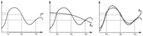
Gradient descent can be used to fit training examples of this type, as explained in [Simard et al., 1992]. Fig. 1 illustrates the utility of this additional slope information in function fitting.
Notice if multiple positive instances are available in X , slopes can be derived from each one. In this case, averaged slopes are used to constrain the target function:
Here Xpos C X denotes the set of positive examples in X . The application of the EBNN algorithm to learning with invariance networks is summarized in Table 2.
Generally speaking, slope information extracted from the invariance network is a linear approximation to the variances and invariances ofF at a specific point in I. Along the invari ant directions slopes will be approximately zero, while along others they will be large. For example, in the aforementioned find-and-fetch tasks, suppose color is an important feature for classification while brightness is not. This is typically the case in situations with changing illumination. In this case, the in variance network could learn to ignore brightness, and hence the slopes of its classification with respect to brightness would be approximately zero. The slopes for color, however, would be large, given that slight color changes imply that the object would belong to a different class.
When training the classification network, slopes provide ad ditional information about the sensitivity of the target func tion with respect to its input features. Hence, the invariance network can be said to bias the learning of the classification network. However, since EBNN trains on both slopes and values simultaneously, errors in this bias (incorrect slopes due to approximations in the learned invariance network) can be overturned by the observed training example values in X. The robustness of EBNN to errors in estimated slopes has been verified empirically in robot navigation [Mitchell and Thrun, 1993] and robot perception [O'Sullivan et al., 1995] domains.
3 Example
3.1 The Domain: Object Recognition
To illustrate the transfer of knowledge via the invariance net work, we collected a database of 700 color camera images of seven different objects (100 images per object), as depicted in Fig. 2 (left columns).
| Object | color | size |
|---|---|---|
| bottle hat hammer can book shoe glasses | green blue and white brown and black red yellow brown black | medium large medium medium depending on perspective medium small |
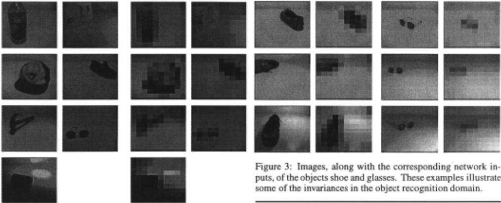
The objects were chosen so as to provide color and size cues helpful to their discrimination. The background of all images consisted of plain, white cardboard. Different images of the same object varied by the relative location and orientation of the object within the image. In 50% of all snapshots, the location of the light source was also changed, producing bright reflections at random locations in various cases. In some of the images the objects were back-lit, in which case they appeared to be black. Fig. 3 shows examples of two of the objects, the shoe and the glasses.
Images were encoded by a 300-dimensional vector, provid ing color, brightness and saturation information for a down scaled image of size 10 by 10. Examples for the down-scaled images are shown in Figures 2 (right columns) and 3. Although each object appears to be easy to recognize from the original image, in many cases we found it difficult to visually classify objects from the subsampled images. However, subsampling was necessary to keep the networks to a reasonable size.
The set of target functions, F, was the set of functions that recognize objects, one for each object. For example, the indicator function for the bottle, /bottle. was 1, if the image showed a bottle, and 0 otherwise. Since we only presented distinct objects, all sets of positive instances were disjoint. Consequently, F obeyed the invariance property. The set of hypotheses H was the set of all artificial neural networks with 300 input units, 6 hidden units, and 1 output unit, as such a network was employed to represent the target function.
The objective was to learn to recognize shoes, i.e., f* = !shoe· Five other objects, namely the bottle, the hat, the ham mer, the can and the book, were used to construct the support sets Y . To avoid any overlap in the training set X and the sup port sets in Y, we exclusively used pictures of a seventh object, glasses, as counterexamples for !shoe· Each of the five support sets in Y, Xbottle· Xhat. Xhammer· Xcan and Xbook. contained 100 images of the corresponding object (positive examples) and 100 randomly selected images of other objects (negative examples). When constructing training examples for the in variance network, we randomly selected a subset of I ,000 pairs of images, 800 of which were used for training and 200 for cross-validation. 50% of the final training and cross-validation examples were positive examples for the invariance network (i .e., both images showed the same object), and the other 50% were negative examples. The invariance network was trained using the Back-Propagation algorithm 2 After training, the invariance network managed to determine whether or not two objects belong to the same class with 79.5% generalization accuracy. It also exhibited 67.0% accuracy when tested with images of shoes and glasses.
2 The classification accuracy of the invariance network was sig nificantly improved using a technique described in [Suddarth and Kergosien, 1990]. See [Thrun and Mitchell, 1994] for details.
3.2 Learning to Recognize Shoes
Having trained the invariance network, we were now inter ested in training the classification network, !shoe· The network employed in our experiments consisted of 300 input units, 6 hidden units, and 1 output unit-no effort was made to opti mize the network topology. A total of 200 examples of images showing the shoe and the glasses were available for training and testing the shoe classification network. In our first exper iment, we trained the classification network using only two of these: a randomly selected image of the shoe (positive exam ple), and a randomly selected image of the glasses (negative example). Slopes were computed using the previously learned invariance network. 3
Our experiments mainly addressed the following two ques tions, which are central to the lifelong learning framework and the invariance approach:
- How important are the support sets, i.e., to what extent does the invariance network improve the generalization accuracy when compared to standard supervised learning?
- How effectively can EBNN overcome errors in the invari ance network? How does EBNN compare to using the in variance network as a learned, generalized distance metric (cf Eq. (4))?
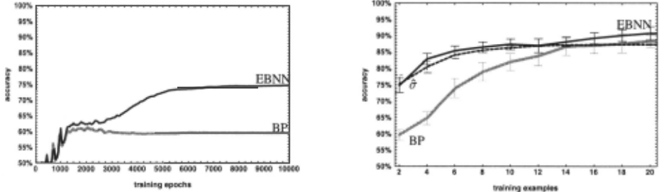
Fig. 4a shows the average generalization curve as a function of training epochs with and without the invariance network. The curve shows the generalization accuracy of the classifica tion network, each trained using one positive and one negative example. Without the invariance network and EBNN, the av erage generalization accuracy for Backpropagation is 59.7%. However, EBNN increases the accuracy to 74.8%. The in variance network alone, when used as generalized distance metric, classifies 75.2% of unseen images correctly. Notice the accuracy of random guessing would be 50.0%.
3 Since in our experiment the negative class, i.e. , the glasses, forms itself a disjoint class of images, those images are also used to de rive slopes (the slopes of u were simply multiplied by -I). This effectively doubles the number of slopes considered in Eq. (5). The corresponding probabilities I - u( i , incg) can also be incorporated into Eq. (4). See [Thrun and Mitchell, 1994] for details.
The difference between the performance with and without support sets, which is statistically significant at the 95% level, can be assessed in several ways. In terms of residual error, Backpropagation exhibits a misclassification rate that is 60.1% larger than that of EBNN. A second interpretation is to look at the performance increase, which is defined as the difference in classification accuracy after learning and before learning, assuming that the accuracy before learning is 50%. EBNN's performance increase is 24.8%, which is 2.6 times better than Backpropagation's 9.7%. On the other hand, the difference between EBNN and the invariance network is not statistically significant (at the 95% confidence level).
Each of these numbers has been obtained by averaging 100 experiments. Examining a single experiment provides addi tional insight. For example, when the neural network is trained using the single image of the shoe and the single image of the glasses depicted in Fig. 2, plain Backpropagation classifies only 52.5% ofthe test images correctly. Here the generalization rate is particularly poor, since the location of the objects within the image differs, and Backpropagation mistakenly considers location the crucial feature for object recognition. EBNN pro duces a network that is much less sensitive to object location, resulting in a 85.5% generalization accuracy in this particular experiment.
Notice that the results summarized above refer to the classi fication accuracy after 10,000 training epochs, using just one positive and one negative training example. As can be seen in Fig. 4a, Backpropagation suffers from some over-fitting, as the accuracy drops after a peak at about 2,050 training epochs. The average classification accuracy at this point in time is 61.3%. However, due to lack of data, it is impossible in this domain to use early stopping methods that rely on cross validation, and it is not clear that such methods would have improved the results for Backpropagation significantly.
These results illustrate that support sets can significantly boost generalization accuracy when training data for the target function is scarce. They also illustrate that EBNN manages to make very effective use of the invariance knowledge cap tured in fr. Results for experiments with larger training set sizes are depicted in Fig. 4b. As the number of training exam ples increases, Backpropagation approaches the performance of EBNN. After presenting 10 randomly drawn training ex amples of each class, EBNN classifies 90.8% and Backprop agation classifies 88.4% of the testing data correctly. This matches our expectations, as the need for background knowl edge decreases as the number of training examples increases. The invariance network alone using Eq. (4) (dashed curve) performs slightly worse than both of these methods. Its gener alization accuracy is 87.3%, which is significantly worse than that ofEBNN (at the 95% confidence level).
3.3 The Role of the Invariance Network
The improved classification rates ofEBNN, which illustrate the successful transfer of knowledge from the support sets via the invariance network, raise the question of what exactly are the invariances represented in this network. What type information do the slopes convey?
A plausible (but only approximate) measure of the impor tance of a feature is the magnitude of its slopes. The larger the slopes, the larger the effect of small changes in the feature on the classification, hence the more relevant the feature. In order to empirically assess the importance of features, average slope magnitudes were computed for all input pixels, averaged over all 100 pairs of training instances. The largest average slope magnitude was found for color information: 0.11. In comparison, saturation slopes were, on average, only 0.063 (this is 57% of the average for color slopes), and brightness slopes only 0.056 (51%).
These numbers indicate that, according to the invariance net work, color information was most important for classification. To verify this hypothesis, we repeated our experiments omit ting some of the image information. More specifically, in one experiment color information was omitted from the images, in a second saturation, and in a third brightness. The results
| without inv. net | with inv. net | |
|---|---|---|
| no color | 52.4% | 57.9% |
| no saturation | 59.0% | 72.9% |
| no brightness | 58.7% | 76.3% |
| full information | 59.7% | 74.8% |
confirmed our belief that color information indeed dominates classification. It is clear that without color the generalization accuracy over the test set is poor, although EBNN still general izes better. If saturation or brightness is omitted, however, the generalization rate is approximately equivalent to the results obtained for the full images reported above. However, learning required significantly more training epochs in the absence of brightness information (not shown here).
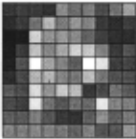
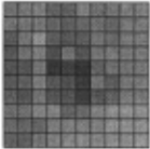
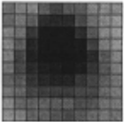
Fig. 5 shows average slope matrices for the target category (shoes) with respect to the three input feature classes, measur ing color, brightness and saturation. Grey colors indicate that the average slope for an input pixel is zero. Bright and dark colors indicate strongly positive and strongly negative slopes, respectively. Notice that these slopes are averaged over all 100 explanations used for training.
As is easily seen, average color slopes vary over the im age, showing a slight positive tendency on average. Average saturation slopes are approximately zero. Brightness slopes, however, exhibit a strong negative tendency which is strongest in the center of the image. One possible explanation for the lat ter observation is the following: Both the shoe and the glasses are dark compared to the background. Shoes are, on average, larger than glasses, and hence fill more pixels. In addition, in the majority of images the object was somewhere near the center of the image, whereas the border pixels showed signif icantly more noise. Lack of brightness in the image center is therefore a good indicator for the presence of the shoe, as is clearly reflected in the brightness slopes derived from the invariance network. The less obvious results for color and sat uration might be attributed to the fact that optimal classifiers are non-linear in color and saturation. To discriminate objects by color, for example, the network has to spot a specific in terval in color space. Hence, the correct slopes can be either positive or negative depending in the particular color of a pixel, cancelling each other out in this plot.
As pointed out earlier, slopes provide first-order information, and invariances may well be hidden in higher-order deriva tives. However, both the superior performance of EBNN and the clear correlation of slope magnitudes and generalization accuracy show that EBNN manages to extract useful invari ance information in this domain, even if these invariances defy simple interpretation.
3.4 Using Support Sets as Hints
A related family of methods for the transfer of knowledge across learning tasks are proposed in [Suddarth and Kergosien, 1990], [Pratt, 1993], [Caruana, 1993]. In a nutshell , these ap proaches develop improved internal representations by consid ering multiple functions in F (sequentially, or simultaneously). Following these ideas, we trained a single classification net work providing the support data as "hints" for the development of more appropriate internal representations. This approach re sulted in 62.1% (20 hidden units), or 59.8% (5 hidden units) generalization accuracy when only a single pair of training in· stances was used. These numbers can directly be compared to the experiments reported above. However, we observed significant overfitting when using this architecture. The peak generalization rate of 70.6% (20 hidden units), or 69.8% (5 hidden units), respectively, occurred after approximately 450 training epochs. This generalization accuracy is significantly higher than that of standard Backpropagation, though not as high as that of the invariance approach with EBNN.
4 Discussion
In the lifelong learning framework, the learner faces a collec tion of related learning tasks. The challenge of this framework is to transfer knowledge across tasks, in order to generalize better from fewer training examples of the target function it self.
This paper investigates a particular type of lifelong learning, in which binary classifiers are learned in a supervised manner. In the approach taken here, invariances are learned and trans ferred using the EBNN learning algorithm. The experimental results provide clear evidence of superior generalization in the object recognition domain, when invariances learned from re lated tasks are used to guide generalization when learning to recognize a new object. However, the the invariance approach relies on several critical assumptions:
- Well-defined invariance functions rest on the assumption that F obeys the invariance property. Note even if the in variance property is not satisfied by F, the support sets can be used to train an invariance network. Even the object recogni tion domain presented above provides an example in which the invariance property may hold only approximately. This is because different objects may look alike in sufficiently coarse-grained, noisy images.
- It is also assumed that functions in F possess certain in variances which can actually be learned by the invariance network. This does not follow from the invariance property. The exact invariances that will be learned depend crucially on the input representation and function approximator used for fr.
- We also assumed that the output space 0 of functions in F is binary. However, this assumption is not essential for the invariance approach. In principle, invariance functions may be defined for arbitrary, high-dimensional output spaces, given that a notion of difference between output vectors is available, as demonstrated in [Thrun and Mitchell, 1994].
In the experiments reported above, all three assumptions were at least approximately fulfilled. We conjecture that the real world offers a variety of tasks where learned invariances can boost generalization. Problems such as face recognition, cur sive handwriting recognition, stock market prediction and speech recognition, possess non-trivial but important invari ances. For example, consider the problem of learning to rec ognize faces of various individuals. Here certain aspects are important for successful recognition (e.g., the distance between the eyes), whereas others are less important (e.g., the direction in which the person is looking). After training on a num ber of individuals, we conjecture that an invariance network might grasp some of these invariances, reducing the difficulty of learning faces of new individuals.
The central question raised in this paper is whether learn ing can be made easier when the learner has already learned other related tasks. Will a system that is "trained" to learn generalize better than a novice learner? This paper provides encouraging results in an object recognition domain. However, most questions that arise in the context of lifelong learning still lack satisfactory, more general answers. We expect that future research in this direction will be important to going beyond the intrinsic bounds associated with learning single isolated functions .
Acknowledgment
This research is sponsored in part by the National Science Foundation under award IRI-9313367, and by the Wright Laboratory, Aeronautical Systems Center, Air Force Ma teriel Command, USAF, and the Advanced Research Projects Agency (ARPA) under grant number F33615-93-1-1330. Views and conclusions contained in this document are those of the authors and should not be interpreted as necessarily rep resenting official policies or endorsements, either expressed or implied, of NSF, Wright Laboratory or the United States Government.
@inproceedings{ijcai1995p157,
  title     = {Learning One More Thing},
  author    = {Thrun, Sebastian and Mitchell, Tom M.},
  booktitle = {Proceedings of the Fourteenth International Joint Conference on
               Artificial Intelligence, {IJCAI-95}},
  publisher = {International Joint Conferences on Artificial Intelligence},
  editor    = {Chris S. Mellish},
  pages     = {1217--1224},
  year      = {1995},
  note      = {Learning},
  url       = {https://ijcai.org/proceedings/1995/157},
}
TY - CPAPER TI - Learning One More Thing AU - Thrun, Sebastian AU - Mitchell, Tom M. T2 - Proceedings of the Fourteenth International Joint Conference on Artificial Intelligence, IJCAI-95 PB - International Joint Conferences on Artificial Intelligence PY - 1995 SP - 1217 EP - 1224 UR - https://ijcai.org/proceedings/1995/157 ER -Copied
Machine-readable versions of this paper, for tools and AI agents:





