A Reinforcement Learning Approach to job-shop Scheduling

1 Introduction

Many problems of commercial interest- including job shop scheduling-are instances of NP-Complete prob­ lems. Hence, there is little hope of finding general­ purpose solutions to these problems. However, in any particular application setting, there are usually domain­ specific constraints and regularities that can be exploited to construct fast, domain-specific heuristic algorithms. While such domain-specific heuristics can be engineered by hand , the process is expensive and t ime-consuming. The goal of the research described in this paper is to ex­ plore the possibility of applying reinforcement learning algorithms to discover good domain-specific heuristics automatically.

Reinforcement learning algorithms learn policies for state-space problem-solving tasks. For each state, the policy specifies what action should be performed. Dur­ ing learning, the learning system receives a reinforce­ ment signal (called a "reward") after each action. The Thomas G. Dietterich Department of Computer Science Oregon State University Corvallis , Oregon 97331-3202

U. S. A.

goal of the learning system is to find a policy that maxi­ mizes the expected reinforcement over future actions. In the context of job shop scheduling, the policy tells what scheduling action to make next in order to maximize some measure of the quality of the final schedule.

In this paper, we focus on the application domain of space shuttle payload processing for NASA. The goal is to schedule a set of tasks to satisfy a set of temporal and resource constraints while also seeking to minimize the total duration (makespan) of the schedule. Of particular interest to NASA are scheduling methods that can also be used to repair a schedule when some unforeseen diffi­ culty arises. In previous work on this task, Zweben and colleagues [Zweben et al. , 1994] developed an iterative repair-based scheduling procedure that combines a set of heuristics with a simulated annealing search procedure. The resulting scheduling system provides an efficient and flexible facility for scheduling space shuttle ground op­ erations. It is in regular use at the Kennedy Space Cen­ ter [Deale et al. , 1994] . The challenge for a learning approach is to discover scheduling heuristics that can match or exceed the quality and efficiency of this itera­ tive repair method.

In the remainder of the paper, we describe the scheduling task in greater detail. We then briefly de­ scribe Zweben's iterative repair-based scheduler . Follow­ ing this, we review the reinforcement learning method known as TD(>..) and describe how the scheduling task can be formulated so that TD(>..) can be applied. We then describe our experiments on simulated problem sets and discuss the results . These results indicate that re­ inforcement learning can outperform the iterative repair scheduler on realistic scheduling tasks. Furthermore, the knowledge learned through reinforcement learning can be applied to scheduling problems that are larger and more complex than the ones that were studied during training. These initial results suggest that reinforce­ ment learning has an important role to play in devel­ oping high-performance AI scheduling systems.

2 The NASA Domain and the Iterative Repair Method

The NASA space shuttle payload processing (SSPP) do­ main requires scheduling the various tasks that must be performed to install and test the payloads that are placed in the cargo bay of the space shuttle. In job­ shop scheduling terminology, each shuttle mission is a job. Each job consists of a partially-ordered set of tasks that must be performed. Each task has a duration and a list of resource requirements. For example, the task MISSION-SEQUENCE-TEST has a duration of 7200 andre­ quires two quality-control officers, two technicians, one ATE, one SPCDS, and one HITS. There are 35 different types of resources. There may be many units of a re­ source available. For example, there are 8 quality con­ trol officers available and 25 technicians. However, these available resources may be split into resource pools, so that, for example, the 8 quality control officers might be subdivided into three pools of size 2, 2, and 4. If a task requires two quality control officers, they must both be drawn from the same pool. Resource pools model multi­ ple work shifts and multiple physical locations. A com­ plete schedule must specify the start time of each task and the resource pool by which each resource require­ ment of each task is satisfied.

A typical SSPP problem involves the simultaneous scheduling of between two and six shuttle missions; each mission involves between 32 and 164 tasks. Hence, the SSPP domain requires solving scheduling problems con­ taining several hundred tasks. Most of these tasks must be performed prior to launch, but some also take place after the shuttle has landed. Each shuttle mission has a fixed launch date, but no starting date or ending date. Hence, tasks prior to launch have deadlines but no ready times; tasks after landing have ready times but no dead­ lines. A key goal of the scheduling system is to minimize the total duration of the schedule. This is much more challenging than simply finding a feasible schedule.

Zweben et al. 1994 developed the following iterative re­ pair method for solving this scheduling problem. First, a critical path schedule is constructed by working back­ ward and forward from the launch and landing dates. Each task prior to launch is scheduled as late as the tem­ poral partial order will permit; each task after landing is scheduled as early as the temporal partial order will per­ mit . Resource constraints are· ignored; resource requests are randomly assigned to resource pools. This critical path schedule can be constructed very efficiently, and it provides the starting state for the scheduling problem space. In each state of this problem space, there are two possible operators that can be applied. The REASSIGN­ PooL operator changes the pool assignment for one of the resource requirements of a task. It is only applied when the pool reassignment would allow the resource re­ quirement to be successfully satisfied. The MovE opera­ tor moves a task to a different time and then reschedules all of the temporal dependents of the task using the crit­ ical path method (leaving the resource pool assignments of the dependents unchanged). The MovE operator is only applied to move a task to the first earlier or the first later time at which the violated resource requirement can be satisfied.

These two operators are applied by the iterative repair method as follows. At each step, the earliest constraint violation (i.e. , where a resource pool is over-allocated) is identified. If a REASSIGN-POOL operator can be applied to reduce this over-allocation, then it is applied. If not, then the MovE operator is applied to move one of the offending tasks to an earlier or later time. If several dif­ ferent pool reassignments are possible, one is chosen at random. If both an earlier and a later move are possi­ ble, then one is chosen at random. Of the several tasks involved in the resource violation, one is chosen at ran­ dom based on a heuristic that prefers to move the task that (a) requires an amount of resource nearly equal to the amount that is over allocated, (b) has few tempo­ ral dependents, and (c) needs to be moved only a short distance to satisfy the resource request .

The overall control structure of the algorithm applies simulated annealing to minimize the number of resource pool violations. After each operator is applied, the num­ ber of violations in the resulting schedule is computed. If this has decreased, the resulting schedule is accepted as the "current" schedule. If it has increased, the resulting schedule is accepted only with probability exp( -.6. V /T), where .6. V is the change in the number of violations and Tis the current temperature. The temperature is gradu­ ally decreased. Search proceeds until no constraints are violated. To obtain a short schedule, the algorithm is run several times, and the shortest resulting schedule is selected.

3 Reinforcement Learning, Temporal Difference Learning, and Scheduling

Reinforcement learning methods learn a policy for select­ ing actions in a problem space. The policy tells for each state which action is to be performed in that state. After an action a is chosen and applied in state s , the problem space shifts to state s' and the learning system receives reinforcement R(s , a, s').

To view the scheduling problem as a reinforcement learning problem, we must describe the problem space and the reinforcement function R . We employ the same problem space as Zweben et al. The starting state s0 is the critical path schedule as discussed above. We define the reinforcement function R(s, a, s') to give a reinforcement of -0.001 for each schedule s' that still contains constraint violations. This assesses a small penalty for each scheduling action (REASSIGN-POOL or MovE), and it is intended to encourage reinforcement learning to prefer actions that quickly find a good sched­ ule. For any schedules' that is free of violations, the rein­ forcement is the negative of the resource dilation factor, -RDF(s', s0). The RDF attempts to provide a scale­ independent measure of the length of the schedule, and this final reinforcement is intended to encourage rein­ forcement learning to find short final schedules. Because the reinforcement function depends only on the resulting state, we will write it as R(s').

The RD F is defined as follows. Let capacity( i) be the (fixed) capacity ofresource type i- that is, the combined capacity of all resource pools of resource type i. At each timet in the schedule, let u( i, t) be the current utilization of resources of type i. If u(i, t) > capacity(i), then the resource of type i is overallocated at time t (no matter how we assign resource requests to resource pools of this type) . We define the resource utilization index RU I( i, t)

for resource type i at time t to be

If the resource is not over-allocated, RU I(i, t) is 1; oth­ erwise it is the fraction of overallocation.

The total resource utilitization index (T RU I) for a schedule of length I is the sum of the resource utiliza­ tion index taken over all n resources and all I times:

Given these definitions , the resource dilation factor 1s defined as

To understand the rationale behind this formula, first note that in the final schedule s, T RU I ( s) is just n times the length of the schedule. This is because in the final schedule, no resource is overallocated, so RU I( i, t) = 1. Hence, T RU I( s) = I x n. We could have used the neg­ ative of this value as the reinforcement function, but re­ inforcement learning is easier if the reinforcement func­ tion is independent of the difficulty of the scheduling problem. A very difficult problem (e.g., with many jobs that have simultaneous deadlines) would require a very long schedule, whereas a simple problem would require a much shorter schedule. The total resource utilization index of the initial schedule, TRUI(s0 ), measures the amount of overallocation of resources in the initial state, and hence, provides a crude measure of the difficulty of the scheduling problem. Hence, we use this to normalize the final schedule length to produce the resource dilation factor .

Now that we have specified how to view repair-based scheduling as a reinforcement learning problem, we turn our attention to the learning algorithm. Suppose at a given point in the learning process we have developed policy 1r, which says that in state s the best action to select is a = 1r( s). We can define an associated function f", called the value function, such that f" ( s) tells the cu­ mulative reward that we will receive if we follow policy 1r from state s onward. Formally, f"(s) = Ef=o R(sj+1), where N is the number of steps until a conflict-free sched­ ule is found.

As in most reinforcement learning work, we will at­ tempt to learn the value function of the optimal policy 7r*' denoted r = !1f·' rather than directly learning 7r*. Once we have learned this optimal value function, we can transform it into the optimal policy via a simple one-step lookahead search: To choose the best action in state s, we compute the state a(s) that would result from applying each possible action a to states. For each such action, we compute the value of the resulting state, r (a( s))' and choose the action a that maximizes this value. Note that this approach requires that we know the effects of our operators-which is certainly true for repair-based scheduling operators.

To learn the value function, we can apply the method of temporal difference learning known as T D( >.) devel­ oped by Sutton 1988. In TD(>.), the value function is represented by a feed-forward neural network, /(s , W) , where W is the vector of weights in the network. If the policy 1r were fixed, T D( >.) could be applied to learn the value function /pi as follows . Let so, s1, . .. , SN be a sequence of states visited by following policy 1r with as­ sociated reinforcements R( s1) , .. . , R( s N) . At step j + 1, we can compute the temporal difference error at step j as

T D(>.) then computes the smoothed gradient

and updates the weights of the network according to

Here, >. is a smoothing parameter that combines previous gradients with the current gradient in ej, and a is the learning rate.

The T D( >.) algorithm was designed to learn the value function for a stationary Markov random process such as would result from following a fixed policy. In reinforce­ ment learning, however, we want to apply it to learn the value function of the optimal policy starting with an initial, random policy. To do this, we employ a form of value iteration. TD(>.) is applied online to the sequences of states and reinforcements that result from choosing ac­ tions according to the current estimated value function, /. At each state s during learning, we conduct a one­ step lookahead search using the current estimated value function j to evaluate the states resulting from apply­ ing each possible operator. We then select the action that maximizes the predicted value of the resulting state s'. After applying this action and receiving the reward , we update our estimate of j to reflect the difference be­ tween the value of /(s) and the more informed value R(s') + /(s'). (We actually employ a slightly more com­ plex procedure described below.) This means that the policy is continually changing during the learning pro­ cess . Fortunately, T D( >.) will still converge under these conditions [Sutton, 1988].

There are five further modifications that we made to this algorithm based on preliminary experiments . First , for any reinforcement learning algorithm it is critical to perform some kind of exploration to discover new and better ways of getting from the start state to the goal. We employed the following simple exploration strategy. At each state, with probability (J we choose a random action instead of the action recommended by the current value function and policy. Initially, (J is set to 1. After each action, (J is decreased by an amount ~(J until it reaches a final value of 0.05. (The values used for ~(J are given below.)

Second, we do not perform weight updates in the neu­ ral network after each action. Instead, we remember the sequence of states visited along the path from the start­ ing state to the final conflict-free schedule. Then we up­ date the network starting with the final action and work­ ing backward to the start of the action sequence. Exper­ imentally, this works better than simple online training, because the values being backed up are more up-to-date.

Third, we employ Lin's experience replay method. During learning, the best sequence of moves from start to goal is remembered, and after every four training se­ quences, we update the network using this best training sequence. This improved learning and performance sig­ nificantly.

Fourth, we do not employ a full one-step lookahead search to select actions, because the branching factor in this problem space is typically 20, and it is costly to compute the value of each of these 20 successor states. Instead, we employ random sample greedy search, which generates a random subset of the possible operators and evaluates their resulting states. The best of these oper­ ators is then chosen. The size of the random sample is determined incrementally. An initial sample of four ac­ tions is chosen. Based on the resulting computed values and a permitted amount of error f. and desired confidence 1- 8, we can compute the probability that the value of the best sampled action is within f. of the best possible action. We continue sampling possible actions until this probability exceeds 1- 8 (we set f. = 0.1 and 8 = 0.1) . Random-sample greedy search is employed during both training and execution .

The final change in the learning algorithm is that we do not use the actual states of the scheduling process as input to the neural network . The neural network can accept only a fixed vector of feature values describing each state (i .e., each current schedule) . Schedules, on the other hand, are variable-length objects. Hence, it was necessary to define a set of useful features that extract important aspects of the current schedule that the neural network can use to predict the value of the state. We defined the following features (based on a very modest amount of experimentation):

Mean and standard deviation of the free pool capacity for bottleneck pools: Simple experiments showed that only the technician, logistics, electrical en­ gineer, mechanical engineer, and quality control officer resource types became major bottleneck resources. For each bottleneck pool, the number of unallocated units (the free capacity) is measu-red over the whole sched­ ule period and the mean and standard deviation of this quantity provide two features for each pool.

Mean and standard deviation of slacks: The slack time between a task and one of its temporal prereq­ uisites is the difference between the end time of the pre­ requisite task and the scheduled start time of the task. We measure the minimum slack for each task (and all of its temporal prerequisites) and the average slack for each task. The mean and standard deviation of these two quantities taken over all tasks provide four features.

Modified RDF: We used a slightly modified version of the resource dilation factor of the current schedule. The numerator of the modified RDF is computed using the capacity and allocation of individual resource-pools rather than of resource types.

Over-allocation index: This is the total number of units of over-allocated resources in the current schedule divided by the total number of units of over-allocated resources in the starting schedule.

Percentage of windows in violation: A window is defined to be a maximal period of time during which the set of currently scheduled tasks does not change. A schedule can be segmented into a sequence of windows. We compute the percentage of windows that contain a constraint violation. We also find the earliest window that contains a constraint violation and compute the per­ centage of the following 9 windows that have violations.

Percentage of windows in violation that can be resolved by pool reassignment: This is the fraction of those windows having constraint violations where the total amount of resources assigned is actually less than the total capacity, so that-if the resources were not sub­ divided into pools-the resource requirements could be met .

Percentage of time units in violation: This is measured over the whole schedule period.

First violated window index (normalized): Let w0 be the index of the earliest window that has a viola­ tion. Let W be the total number of windows. Then this feature is (W- w0 )/W. As violations are repaired, this value decreases to zero. If no window has a violation, we set wo = W .

Each of these features was developed by studying small scheduling problems to find quantities that had some ability to predict RDF. However, we believe that these features can be improved substantially, and this is a goal of our ongoing research.

A consequence of using these features instead of the full state is that the learned policy may enter infinite loops. We have taken two steps to detect and prevent these loops. First, the randomness introduced by the random sample greedy procedure and by the random exploration process tends to avoid loops, because even when the same state is revisited, the same action may not be chosen. Second, all states visited while solving a particular problem are recorded and checked to detect loops. When a loop is detected, we apply the learned value function to compute the second best action and choose it. If a loop is detected again at the same state, we backtrack to the preceeding state and again take the second best action. If this were to create a loop also, we would continue backtracking to earlier states.

4 Methods

We briefly describe the methods applied to generate the training and test problems, the network architecture, and the parameters employed in the learning algorithm.

4.1 Problem Sets

We constructed two problem sets: an artificial prob­ lem set and a problem set based on specifications for the NASA SSPP problem. The artificial problems were generated as follows. First, we generated a pool of 20 jobs. From these, we constructed scheduling problems by choosing random subsets ofthese jobs. This was in­ tended to model the NASA setting where there are only a limited number of possible shuttle-cargo-bay configura­ tions (i.e., jobs), but where each scheduling problem is a unique combination of such shuttle missions. More gen­ erally, this models a job shop where each new scheduling interval requires scheduling a unique mix of more-or-less standard jobs.

To generate a synthetic job, we choose the number of tasks randomly in the range 6 to 10. A set of tem­ poral constraints among these tasks is then randomly generated such that approximately 60% of all possible pairwise precedence constraints are asserted.

Next , resource requirements are determined for each task. There are two types of resources. Each resource has two pools-one pool has a capacity of 6 units, and the other has a capacity of 8 units. Resource require­ ments are randomly assigned to each task uniformly in the range from 0 to 6 units for each resource type .

Once the pool of 20 jobs is generated in this way, 50 training problems and 50 test problems are constructed. To generate a problem, we first choose the number of jobs in the problem to be either 3 or 4 (with equal prob­ ability) . The desired number of jobs is selected ran­ domly with replacement from the 20-job pool. Each job is assigned a completion deadline with the deadlines ran­ domly separated by between 8 and 15 time units.

Sixteen input features are computed to represent schedules for these problems: 8 pool capacity features for the 4 pools, 4 slack features, and features describ­ ing the modified RDF, percentage of windows and time units in violation, and percentage of violated windows in which the violation can be resolved by pool reassign­ ment .

During training, 15 of the 50 training problems were held out as a validation set to determine when to halt training. The remaining 35 problems were repeatedly processed to train the value function networks.

In addition to the 50 test problems, we generated a second test set of 20 larger problems to evaluate the abil­ ity of the learned value functions to scale up to larger scheduling problems. Each of these larger problems was generated in the same way as the smaller problems ex­ cept that the number of jobs was chosen uniformly be­ tween 15 and 20.

For the space shuttle payload processing task, a prob­ lem consists of a set of shuttle missions with launch dates one to three months apart. Each mission can have one or two payloads. We considered three kinds of payloads: long module (LM), mission peculiar equipment support structure (MPESS), and pallet and igloo (PALLET & IGLOO). These have 65, 32, and 82 tasks, respectively. There are 35 types of resources of which only five are major bottleneck resources.

We randomly generated a training set of 20 problems and a test set of 20 problems. The training problems each contained between two and four shuttle missions. Of the 20 training problems, 5 were held out for valida­ tion to determine when to stop training. The test prob­ lems each contained 3 to 6 shuttle missions. The test problems thus assess the ability of the learned policy to scale up to larger problems.

For the shuttle problems, 20 input features are used: 10 features for pool capacity, 4 slack features, modified RDF, 2 features describing windows in violation, per­ centage of time units in violation, index of first violated window, and the over allocation index.

4.2 Network Architecture and Training Procedure

To represent the value function, we trained feed-forward networks having 40 sigmoidal hidden units and 8 sig­ moidal output units. The 8 output units encode the pre­ dicted RDF using the technique of overlapping gaussian ranges [Po!Ilerleau, 1991) as follows . Each output unit represents one assigned RDF value, Vj (j = 1, . .. , 8) . For the artificial problems, these RDF values are VI = 0.8 , v2 = 1.0, . .. , v8 = 2.2. For the SSPP problems, the RDF values are VI = 0.9, v2 = 1.0, ... , vs = 1.6. During training, the target output activation for each output unit is set to be targetj = <p(RDF- Vj ,0.2)j<p(0 ,0.2) , where <p(J.l, u) is the standard normal probability den­ sity function with mean J.l and standard deviation O" . During testing, the predicted RDF value is computed as o:::::j actj · Vj)j("L_j actj ), where actj is the actual output activation for output unit j.

For each problem, we trained eight different net­ works using all combinations of the following parame­ ters: learning rate a= 0.1 or 0.05, exploration schedule 1}.{3 = 0.001 or 0.0005, and A = 0.2 or 0.7. (Prelimi­ nary experiments showed that A = 0 did not perform as well.) The training set problems are processed in round-robin fashion . Each problem is solved using one of the networks to obtain a sequence of states and ac­ tions . That network is then updated (via backpropaga­ tion with TD(A)) by processing the state sequence work­ ing backward from the final state. After every 50 passes through the training set, a cross-validation test is con­ ducted to compute the average RDF of the final sched­ ules produced over all cross-validation problems . The best network found during cross-validation (for each of the eight parameter sets) is retained. For each network , training continues until the cross-validated RDF of that network is worse than the previous nine measured values for cross-validated RDF.

Six networks are chosen for testing as follows . The three best networks found during cross-validation are re­ tained along with their corresponding final networks . We retain the final networks to compensate for variance in the cross-validation measurements.

For the simulated annealing component ofthe iterative repair method, we set the starting temperature to 100 for the synthetic scheduling task and to 200 for the SSPP task. After every 10 accepted repairs to the schedule, the temperature is reduced according to T := 0.95T.

5 Results

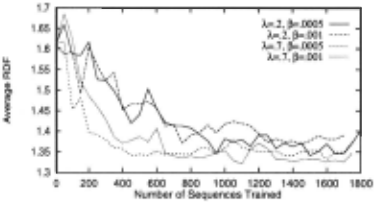
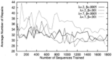
Figure 1 shows the average cross-validation RDF for the four value function networks trained with a = 0.1. The horizontal axis gives the number of training sequences processed. This figure shows that the performance of the trained networks is improving on the cross-validation problems. Figure 2 plots the number of repair actions for these same networks. This shows that there is some reduction in the number of actions required to convert the starting schedule into a conflict-free final schedule.

Figures 3 compares the performance of temporal dif­ ference (TD) scheduling with the iterative repair (IR)

method ofZweben. The vertical axis is the RDF of the best conflict-free schedule found so far . The horizontal axis is a machine-independent proxy for the amount of CPU time consumed by each method. For IR, the hori­ zontal axis gives the number of restarts of the simulated annealing procedure, and the vertical axis records the RDF of the best conflict-free schedule found so far. The longer IR is run , the better its performance.

For the TD scheduler, the horizontal axis represents the number of neural network evaluation functions em­ ployed. When k networks are used to solve a schedul­ ing problem, the problem is solved k times, once with each network, and the schedule having the best RDF is returned as the answer. The best k networks as deter­ mined by cross-validation, are used. The cur~es stop at k = 6, because only six networks were used (once each).

~orne care must be taken in interpreting the horizontal ax1s as a measure of CPU time. Each step of the TD scheduler requires more CPU time than a step of the IR scheduler , because the TD scheduler must perform the random sample lookahead search and check for loops. On the average , TD spends 2.2 times as much CPU time per step as IR. On the other hand, TD requires fewer steps to find a conflict-free schedule. The average sequence length for an iteration of TD is 82% as long as an average IR sequence. The net effect is that one iteration of TD is equivalent to approximately 1.8 iterations of IR.

Bearing this in mind, the key point to notice is that the curve for the TD scheduler always lies below the curve for iterative repair. This means that given the same amount of. CPU time, TD always finds a better schedule (i.e., w1th lower RDF). For example, with 6 networks TD ob­ tains an RDF of 1.320 compared to IR's RDF 'or 1.371 (at.1.8.·6 = 11 iterations). This is a 3.9% improvement, wh1ch m a schedule lasting a year is a savings of 14 days

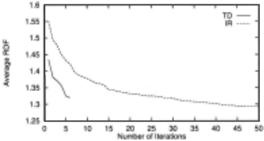
(and thousands of dollars) . The curve also shows that it~rative repair always requires much more time (29 iter­ atwns vs . 11) to find a schedule whose quality matches the RDF found by TD.

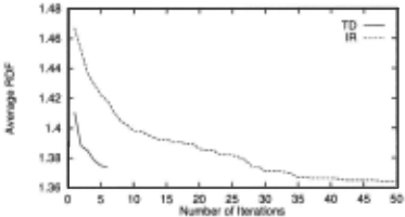
Figure 4 shows a similar comparison for TD and IRon the 20 larger test problems. Here the difference between the algorithms is even more pronounced. Temporal dif­ ference ~cheduling scales be!ter to larger problems, even though 1t has only been tramed on smaller problems.

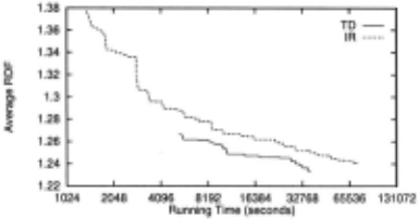
Figure 5 shows analogous results for temporal differ­ ence and iterative repair on the 20 test-set SSPP prob­ lems. Here the horizontal axis is log CPU time. We see that TD maintains a constant factor advantage over iter­ ative repair. Temporal difference scheduling finds better schedules faster than iterative repair.

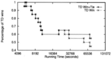
Note, however, that this figure just gives the average RDF over the whole test set . Because of the random components of both algorithms, this hides considerable variation. Figure 6 reveals this variation. Let us say that TD "wins" on a particular problem if the RDF of its best schedule computed so far is better than the RDF of the best IR schedule computed with the same amount of CPU time. The two algorithms will be said to "tie" if they find schedules with identical RDF values. Figure 6 plots the fraction of TD "wins" and TD "wins + ties" as a function of log CPU time. We see that at low CPU costs, TD wins on almost every problem. Eventually, as CPU time becomes larger, TD still wins or ties slightly more than 50% of the time.

6 Discussion and Concluding Remarks

These results show that temporal difference (TD) meth­ ods outperform the best previous algorithm for schedul­ ing space shuttle payload processing jobs. Furthermore, there are clearly many ways that the TD methods can be improved. For example, the current set of features needs to be improved so that the learning procedure can cap­ ture more domain-specific knowledge. There is also some evidence to suggest that the training procedure could be improved.

Several authors [Bradtke, 1993; Thrun and Schwartz, 1993; Boyan and Moore, 1995; Schraudolph et a/., 1994] have shown that there are pitfalls associated with us­ ing neural networks (and other function approximation schemes) to represent value functions in reinforcement learning. However, the results of this paper and the no­ table success of Tesauro's [1992] TD backgammon sys­ tem show that in some situations, these pitfalls are not encountered. An important open question is to under­ stand why TD(>.) works in this and other applications.

We suspect that the success of TD methods in this domain results from two factors. First, there are prob­ ably many good solutions to each scheduling problem. Certainly there are many good solution paths, because the search space is highly redundant . Second, TD is es­ sentially a technique for smoothing adjacent estimates of the final RDF. This smoothing can remove local minima even if it does a poor job of predicting the final RDF. These two properties may permit a simple greedy algo­ rithm to find good schedules.

These same two properties may explain why the iter­ ative repair method with simulated annealing also suc­ ceeds in this domain. Simulated annealing is a stochastic method for locally smoothing an objective function . As applied in this domain, simulated annealing is not run long enough to find a global optimum, but it may be able to escape local minima and find an acceptable solution in spite of this.

Industrial scheduling problems abound, and general­ purpose solutions to these problems probably do not ex­ ist. This research has shown that reinforcement learn­ ing methods have the potential for quickly finding high­ quality solutions to these scheduling problems. The goal of future research must be to improve these learning methods so that they can be applied with a minimum of domain-specific engineering to produce a new, cost­ effective scheduling technology.

Acknowledgements

The authors thank Rich Sutton and Monte Zweben for several helpful discussions. The authors gratefully ac­ knowledge the support of NASA grant NAG 2-630 from NASA Ames Research Center . Additional support was provided by NSF grants CDA-9216172 and IRI-9204129.