
A Qualitative Discretization for Two-Body Contacts
Proceedings of the Fourteenth International Joint Conference on Artificial Intelligence. Knowledge Representation. Pages 915-922.
© 1995 International Joint Conferences on Artificial Intelligence
Abstract
In this work we use contact alignments as qualitative landmarks to discretize the relative motion between two 3D objects. We use assembly planning as a sample domain, and address the question of obtaining the assembly blocking graphs from the geometry and the motion constraints. Starting from a geometrical description of the objects we characterize contacts involving topologically distinct feature sets, called contact formations (CF), and obtain a qualitative decomposition of the configuration space based on CFs. We show how standard algorithms for finding the configurationspace routinely discard CF information, and how these can be extracted at no additional computational cost. Finally we show how CFs can be used to generate assembly solutions and for correcting jamming and other assembly errors.
- Null 3. ( c, 12), (b, 12), (be, 12)
- A. Bourjault. Contribution a une Approche Method- olodique de L 'Assemlage Automatixe: Elaboration Au- tomatique des Sequence Operatores. PhD thesis, Univer- site de Franche-Comte, Besancon, France, Nov . 1984.
- J . F . Canny. The Complexity of Robot Motion Planning. The MIT Press, Cambridge, 1987.
- Eliseo Clementini and Paolino Di Felice. A comparison of methods for representing topological relationships. In- formation Sciences , to appear.
- L. S. Homem de Mello and A. C. Sanderson. And/or graph representation of all assembly sequences. IEEE Trans . of Robotics and Automation, Vol. (6)(2):188-199, Apr. 1990.
- a, 67), (b, 67), (67, ab) 23. (6, ab), (b, 67), (67, ab) 25 . (b, 56), (6, be), (56, be) 27. (b, 56), (c, 56), (56 , be) 29 . (5 , be), (c, 56), (56, be) 31. (b, 12), (2, be), (be, 12) 33. 32
- Rajiv Desai and Richard A. Volz. Identification and ver- ification of termination conditions in fine motion in pres- ence of sensor errors and geometric uncertainties. IEEE Conference of Robotics and Automation, May 1989. References
- Varol Akman and Paul J. W. ten Hagen. The power of physical representations. AI Magazine, pages 49-65, 1989.
- James F. Allen. Maintaining knowledge about temporal intervals. IEEE PAM!, Vol. 26(11):832-843, November 1983 .
- P. Bhatia. Automatic Robotic Assembly from Disassem- bly: An Approach Using Robot Path Planning. PhD the-
- Boi Faltings. Qualitative kinematics in mechanisms. Ar- tificial Intelligence, Vol. 44{1-2):89-119, 1990. IJCAI
- Kenneth D. Forbus, Paul Nielsen, and Boi Faltings. Qualitative spatial reasoning: the clock project. Arti- ficial Intelligence, Vol. 51:417-471, October 1991.
- Ziv Gigus, J. Canny, and R. Seidel. Efficiently comput- ing and representing aspect graphs of polyhedral objects. [12]
- CACM, Vol. 13(6):542-551, 1991.
- Jean-Claude Latombe. Robot Motion Planning. Kluwer Academic Publishers, Massachussets USA, 1991.
- S. Lee. Backward assembly planning with assembly cost analysis. In IEEE Conference of Robotics and Automa- tion, pages 2383-2391, 1992.
- Amitabha Mukerjee and G. Joe. A qualitative spatial representation based on tangency and alignment. Tech- nical Report 92-003, Texas A&M University CS Dept, Feb 1992. Shorter version in AAAI-90 (p.721-727).
- Amitabha Mukerjee and Nishant Mittal. A qual- itative representation of frame-transformations in 3- dimensional space. Technical Report ME-94-02, liT Kanpur Department of Mechanical Engg, 1994.
- T . Lozano Perez. Spatial planning: A configuration space approach. IEEE Trans . Computers, Vol. (C- 32){2):108-120, Feb. 1983.
- David Pierce and Benjamin Kuipers. Learning to explore and build maps. AAAI-94, pages 1264-1271, 1994.
- J . Rei£. Complexity of the mover's problem and gen- eralizations. In Proc. 20th IEEE Symposium FOGS, 1979. Also in Planning, Geometry and , Complexity of Robot Motion, edited by J. Schwartz, J. Hopcroft and M. Sharir, Ablex publishing corporation, New Jersey, 1987, Ch. 11, pages 267-281.
- Randall H. Wilson and Jean-Claude Latombe. Geomet- ric reasoning about mechanical assembly. Artificial In- telligence, v.72:1-2:371-396, November 1994.
- J. Wolter, S. Chakrabarty, and J . Tsao. Mating constri- ant languages for assembly sequencing planning. IEEE Conference of Robotics and Automation, pages 2367- 2374, May 1992.
References were extracted automatically from the PDF and may contain errors.
Full text extracted automatically from the PDF; figures, tables and equations may differ. The PDF is the version of record.
1 Introduction
Contact preserving motions between spatial objects is a question that is central to qualitative spatial reason ing [1), constructing assembly plans [7), kinematics [10] fine motion planni?g [8), gross motion planning [12), ancl othe~ ta:sks. In this work we use contact alignments as qualitative landmarks to discretize the relative motion between 3D objects. We focus on assembly planning as an example domain, and show how to obtain a search space from geometric and motion constraint considera tions and provide algorithms for the 2-body motion prob lem in any dimension.
Consider a sequence of motions such as: "Incline the peg and trail it along the top face until you find the hole. Align the edges, straighten and insert it. If jammed you may be touching a side wall." Intuitively this in~ valves a decomposition of the motion space between the peg and the hole into regions such as "inclined-peg-topface" "alig d d " " t · ht " " h' , ne -e ges , s raig -peg , touc mg-sidewall" etc. Much of AI is concerned with the problem Robotics Group
Centre for Artificial Intelligence and Robotics Bangalore, India.
e-mail: p bhatia@cair .ernet .in
of how to develop this type of discretization - in the as seT?bly ~roblem, for example, the question is: given two obJects m contact, how can one characterize the relative motion between them into regions that are qualitatively distinct?
Such a discretization is crucial to reducing the size of the sea~ch space for fine motions, which in a general c??figur~t10n space approach results in a topological par titiOn with an exponential number of manifolds [5] and in practice, it is unlikely (PSPACE hard [18]) that one can test the feasibility of the large number of proposals ma.de by the typical assembly sequencers [3] . Compu tatiOnally such a discretization reduces the search from the continuous domain of part configurations to a finite set of contact regions. Furthermore associated charac teristi~s of each region help in cor;ecting errors - e.g. when Jammed, the reason can be found by investigat ing neighbouring contacts (see [8] for an error recovery application).
Yet, surp~isingly little work has been done on the pro cess of findmg such discretizations for general geome tries. In constructing assembly plans one assumes the existence of such a decomposition: 'AND/OR graphs [~), Precedence graphs [4), Backward Assembly Plan mng [13), Assembly Constraint Graph [20), etc. The close~t approach to handling general geometries is that of Wilson and L~tom~e [19], which extends the blocking graph model to Identify a discretization in the transla tion space in t~o dimensions. The model works only for asse~bly, and IS not useful in spatial reasoning, kine matics, or other tasks. Also, it is restricted to 2D and does not handle rotations. Another class of models used in q~alita~ive ~ineJ?atics, also approaches this work by formmg discretizatiOns along the boundaries of the con figuration [9]. However, these approaches discard the intern~l points. of the ~-space, which are necessary for recordmg relative motiOns between faces in 3-D for ex ample, and do not use contact analysis as a mechanism for capturing the discretization in the spatial positions as ~uch. In terT?s of the assembly problem, some special Ized geometnes belonging to classes like nuts on bolts ca~ be analyzed using knowledge-based techniques, but this cannot extend to the general class of geometries, nor c~n the correctness of the knowledge database be verified Without more general purpose algorithms.
In what sense is this a "qualitative" discretization of the spatial 2-body problem? Many applications of QR involve parameter spaces that reduce to one-dimensional points (-,0,+) or intervals on the real line ([2]) . We were encouraged in this work by qualitative models that discretize visibility regions of an object into "aspect graphs" [11], and by recent work on modeling 3D posi tions using a qualitative-quantitative hybrid [15]. Earlier work in modeling contacts, using the name Contact For mations [8], uses boundary features such as edges, ver tices, faces, to generate a search space in error recovery situations. Other models of qualitative spatial reasoning have attempted connections among spatial objects us ing rectangular enclosures or other approximations [6], and have failed to define a clearly defined, usable set of parameters for qualitatively discriminating the inter actions. Cognitive studies of assembly tasks also seem to indicate the importance of "haptic landmarks" which are formed while playing around with the parts prior to actual assembly. Thus just as the alignment orientation provide "visual landmarks" in constructing a qualitative model for recognition, the contact formations provide a qualitative set of haptic landmarks for fine motion, kine matics, and other tasks. In connection with recognizing landmarks, the new statistical learnin~ techniques for finding landmarks is of particular note l17] .
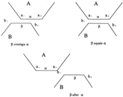
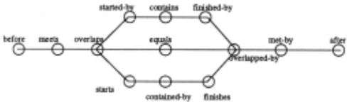
We claim that haptic landmarks are obtained by align ments between boundary features of the objects (such as that involving an edge from one 3D object and a face in another). Such alignments mark regions of change in the contact forces as the set of surface features in contact are altered. For example, considering purely sliding mo tion, we observe that the transitions closely resemble the interval relations well-known in temporal logic and one dimensional qualitative spatial reasoning (fig. 1) . As the edge f3 slides along the edge a and its interval relations change, so does the set of contacts occurring between boundary features in A and B. Thus the f3 overlaps a configuration is characterized by the following contacts:
- vertex a1 and edge f3
- edge a and vertex b2
- edge a and edge f3
This is represented as a contact formatimi with three elemental contacts: {(a1,f3),(a, b2),(a,f3)} The entire set of transitions possible in such motion is illustrated in the transition graph (Fig 2) [14], where the tri-furcation indicates the three possibilities with relative size:
- (a) B smaller than A (starts) (lal > l/31) (a , {3), (a1, b1), (a, b2)
- (b) A equal than B (equals) (lal l/31) (a1, bl), (a,/3), (a2, b2)
- (c) B longer than A . (started-by) (lal < 1/31) (a, {3), (a1, bl), (a2, {3)
Pure sliding motions can be modeled in this way, but what about rotations? One way to map the linear inter val problem to a cyclic space (fig. 3), where alignments between surface features such as vertices and edges pro vide decompositions of qualitative interest. Here also, intervals exhibit the same relations except that "after" and "before" in the transition graph of fig. 2 have been joined to form a circle topology. The CF model can cap ture both the translation model of 1-D intervals as well as the rotation zones between alignment positions. This allows us to handle complex spatial reasoning quenes using the CF model.
To generalize to higher dimensions, we approach the configuration space models, which look at the motion space of two bodies in general. The contact forma tions are then discretizations on the surface of the configuration-space obstacle ([9] [12]) . Next we show how any assembly motion can be expressed as a sequence of contact formations, a concept first explored in [8] in the context of Robot Grasping. Thus the chief contri bution of this work is to extend the contact formation paradigm to the problem of constructing assemblies.
2 Qualitative Contacts
[Def] An object A is a bounded set in En with boundary 8A . About a point on the boundary, any finite neigh bourhood contains points both in A and not in A. A d-fa ce (written as fd) , is a subset of the boundary topo logically mappable onto an open disk in Ed , i.e. a d manifold. Ad-face is bounded by lower order hyperedges that are not contained in the face- e.g. the ( d -1 )-faces, which distinguish it from other d-faces. Typically, some geometric change is associated with the lower order faces; e.g. in polyhedra, 1-faces correspond to slope disconti nuities, and constitute part of the boundary of a 2-face. For object A in En, 8A is decomposable into manifolds of order (n-1) or less; the union of all the faces of orders 0 to (n-1) consitutes the boundary of A: 8A = U{(n-1) faces , (n- 2)-faces , ... , 0- faces}.
[Def) The collection of all the faces of the object (as distinct from their union), is the boundary-list uA = {( n - 1)- faces , (n - 2)- faces, . .. , 0- faces} e.g. in E 2 u A = {fl , fn, where fl are the individual d-faces in A. if a 1 ,a2 E uA then a1 n a2 =¢>and Ua; = 8A Thus for a polygon in E 2 , 8A consists of all the points on its boundary, and is the union of the edges (1-faces) and the vertices (0-faces). The boundarylist uA on the other hand, is merely a list of all its 1-faces and 0-faces.
[Def) The transformation TG traditionally viewed as mapping point B x in frame B into a point Ax in frame A, may also be viewed as a motion that maps an object A onto a congruent object B through the same motion that would map frame A onto frame B. This transfor mation is a function TG = TG (it) of the motion vector it that causes frame A to be coincident with frame B. This motion also describes the configuration of B w.r.t. A. For transformations in E 3 with six degrees of free dom, for example, it may consist of three translations and three rotations.
Configuration Space
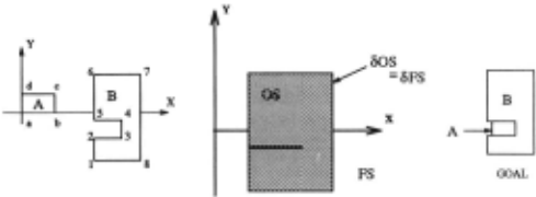
[Def] Configuration space C of a body w.r .t . another is the space of all the configurations it E C the bod ies can have w.r .t . one another. The obstacle space of body B w.r.t . A, OSA(B), is defined as the set of motions that cause a collision between A and B. OSA(B) = {it I 3(x E A)(TG(it)x E B} . 80SA(B) is the boundary of this obstacle space. Figure 4 shows an example of'a 2D translational configuration space for a peg-in-hole assembly task. The bodies A and B are as sumed to be rigid bodies; if an assembly mojion involves deformation, the configuration space approach can only model it by deforming the obstacle space accordingly. A motion path is Contact-preserving iff for any configura tion it on the path, the interiors of the objects do not overlap, but the boundaries touch.
Contact Formations
[Def] A contact A between objects A and B is defined by the d-faces that are in contact , A= {a;, ,Bj} s.t. a ; E uA and ,Bj E u B. A contact formation A is a set of simulta neous contacts, AA(B); = {AI,A2, ... ,An} , where A; are elemental contacts. If the d-faces are chosen to repre sent regions of qualitative continuity (such as the faces of a polyhedron) , then the contact formation (CF) rep resents qualitatively distinguished surface contacts. For simplicity, we will represent AA(B) by A. The contact space .CA(B) is the set of all contact formations of B w.r.t . A.
We observe that the relative positions of the objects that correspond to a CF can be codified by a relative motion vector i1 and the corresponding rigid transfor mation T( it). Thus there exists a mapping from the CF space onto the space of motion vectors.
3 Discretizing the Configuration Space
Lemma la : If i1 E 80S and x E A, y E B s.t. x = TG(il)y, then x E 8A andy E 6B.
Proof' Since it is on the boundary 60S, any finite neighbourhood of it will include configurations both in and not in OS, i.e. 3w, i(w- it)l < f, and w tj_ OS, ie. ('Vy E B)T( w)y tj_ A . Hence ('Vv) I vi < f => (38 > O){T(it+v)y E Ball5[T(it)y]}. Hence Ball6[T(it)y]-A :{; ¢>. But T(it)By E A => T(it)By E 6A => i E 6A. Similarly ii E 8 B.
Lemma lb :Given a configuration it in which the set of points X C A mapped to B by the transformation TG(it) is on the boundary of A, i.e. X C 6A , then the configuration it E 60S.
Proof' Since it results in some points from A being mapped to some points in B, it E (OS) . If it tj_ 60S, then it must be in the interior of the Obstacle Space, i.e. it E int(OS) . But this would imply that there is a ball around it which is contained entirely in OS. This demands that the image of this ball will be a set of points all contained in B, and that the points interior to this ball will not be boundary points on B, which imply that the points in A mapping to these points will also be interior points in A, violating the conditions. Hence iZ E 80S.O
Lemma 2: Vii E 80S A (B), T( u) represents a relative position of A w.r.t. B that represents a unique Contact Formation A E .CA(B).
Proof: Let X C A be the set of points mapped to B by Tff(u), and let Y be its image from B. By Lemma 1, X C 8A and Y C 8 B. X and Y comprise of some subset of d-faces from the boundarylists eTA and CTB. Let any mapped pair of points (x,y) be on the faces (fA.; ,f'JJ), which must be unique by the definition of Objects (no faces overlap). Hence any pair of points defines an el emental contact A which exists and is unique. A finite number of such contacts occurring simultaneously then define a unique Contact Formation A. 0
[Def] Given any Contact Formation A, the Configura tion Patch is a set of configurations r c 80S such that any iZ E r causes a contact in the CF A, and no iZ fi r causes the CF A.
Lemma 3:
1. Any non-null CF A E .CA(B) corresponds to a f; c 80S.
2. Uf; =80S.
3. r; n ri = ¢>, i =F j .
Proof:
1. That all CF's must have a corresponding configura tion patch r follows from lemma 1 b.
2. Let iZ be a configuration s.t. iZ E 80S but iZ fi Uf;. i
By lemma 2, this corresponds to an unique CF A and from part 1 above, this must map to a Configuration Patch r. Hence if iZ E 80S then iZ E U f;. Hence i
3. Say iZ E f; and iZ E ri. Then iZ corresponds to A; and Aj which is not possible since the CF-mapping is unique [Lemma 2].
[Def] Contact Formations A; and Aj with corresponding configuration patches f; and fj are adjacent iff3 (u E f; and v E rj) s.t. a path P exists from iZ to v and P ~ (r, uri)·
For example, in fig. 1, the CFs for 'overlaps' and 'equals' are adjacent, but 'equals' and 'after' are not. The transition graph (fig. 2) can be viewed as a map ping for adjacent relations in one-dimension. Note that 'after' and 'before' are not distinguished in contact for mation space since both are null CFs. Indeed, the null CF corresponds to all configurations where there is no contact, and defines the domain for the gross motion planning problem. It may have disjoint partitions that are not reachable from one another.
Theorem: Two-body contact motions
Given a target configuration with object B in contact with A , if a path to this configuration exists from the the fully separated configuration, then such a path also exists in moving through adjacent Contact Formations.
Proof: The fully separated configuration corresponds to the null CF, and in any assembly process, there will be an initial contact, say u1 . If the remaining assem bly motion remains in contact, then it passes through a sequence of adjacent contact patches f;'s. f; is ad jacent to rj iff the path joining any point off; to any point of ri lies entirely within f; and ri. Since the path is connected such a sequence will always exist. Each f; corresponds to some CF A;. By definition, A; is adjacent to Aj. If there is a contact break, the assembly returns to another null CF, and will, by the same arguments, pass through another sequence of CFs before reaching the CF containing the target configuration. Thus the path hypothesized in the theorem exists. 0
This validates our claim that CFs can be used as a qualitative discretization of the motion space. In the next section we outline the algorithm for determining all CFs, and then we show how the related graph can be searched for determining solution paths to assembly problems.
4 Contact Formations for Polyhedral Objects
A direct algorithm for obtaining all the CF's would be to obtain all contact pairs CT A x CT B, and constrain the objects based on the contacts. If n and m are the car dinalities of CT A and CT B respectively, then there will be 2nm such contact pairs. This is because nm different kinds of elemental contacts are possible and out of these 0, 1, ... , nm may occur simultaneously. However, it is clear that this is a very pessimistic bound, and while it is easy to show tighter bounds for certain classes like convex objects, a more general tighter bound appears difficult to find. For each contact, the constraint space may either be null (impossible contact), or the same as another contact (combine these elemental contacts into a contact formation). Otherwise the CF has only a sin gle contact pair. Constraint propagation is expensive, and we present a more efficient algorithm below. The algorithm is similar to sweep models for obtaining trans lational C-Space, except that instead of discarding the internal structure within the C-Space we now pay par ticular attention to the structure there. We first iden tify all primary contact pairs· which arise due to single feature interactions. Intersections between the primary contact pairs give rise to secondary constraints, which are essentially CFs with more than one elemental pair. The algorithm also returns a graph for the CF space in this translational slice, and the configuration space ob stacle OS can be computed from the CF map, since it is nothing but the outer boundary of the CF map.
[Def] Contact Formation Map n : A discretization on on the surface of the obstacle space of B w.r.t. A in which each region and each bounding face represents a different Contact Formation. The adjacencies between map features relate to adjacencies between their corre sponding CFs.
CF Algorithm: Rotational Alignment Slices
Objective: Given reference object B and secondary object A (A,B E Ed) in a face-alignment configuration (a rotation invariant space), find the CF map n, i.e., all CFs that result from contact preserving motions in this slice. Let the faces in alignment be f'A and /~.
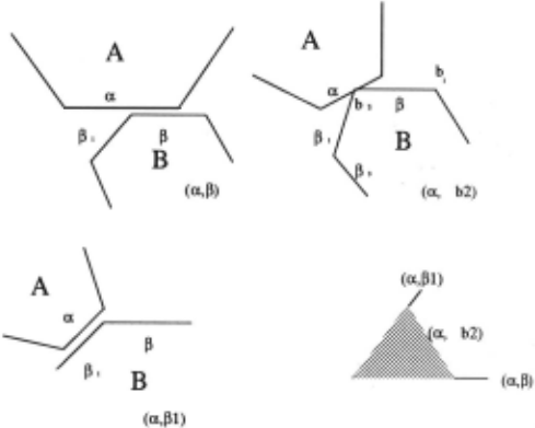
The contact formations in this slice will involve the faces that are in contact, such as the triangular bottom face of the prismatic peg and the top face of the cube in fig. 5a. In this configuration, the two faces are par allel, but also one of the edges of the bottom face is aligned with an edge of the top face; this is not the case in fig.5c. The objective of this algorithm is to find all the CFs possible in this sliding motion. Note that the objects concerned do not have to be convex, and may even include holes.
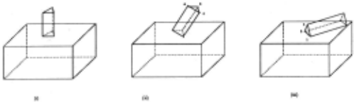
Contact Formation Algorithm for rotational slices
- Record the values and ranges of all the fixed motion variables for this slice. Initialize n to be null.
- Construct the object gA by reflecting every vertex in f'A with respect to the frame of A, and keeping the rest of the polyhedral topology intact. gA is also an r-face. Initialize a vertex g~ 1 as the reference vertex.
- At any vertex f~ on the boundary of the q-face f~ place a translation of the reflected face gA so that the reference vertex gt is coincident with f~ . Add all vertices and edges of this object to n ; e.g. the vertices are: n°(!~) = {w~,w~, ... ,wn = f~U{gA,,gA,, ... }, where the vertices g 0 are taken in the new placement.
- At each w J E no(!~) translate the face f~ such that f~ is coincident with wJ. Add each face of each of these placed objects as a face in n.
- For the original q-face f~, at each vertex !~;, place a translation of the reflected face gA such that the ref erence vertex gt coincides with each /~;. All faces of each of these placed objects (i.e g A's) are added as faces inn.
- The faces added to n so far correspond to ele mental contact, arising from a single contacts. Find all intersections of these elemental contacts to form the set of Contact Formations. Add all intersection sub-faces as faces inn.
Figure 6 shows the result of applying this algorithm to the two faces of fig 5. The prism faces shown by dotted and dashed lines are the critical configurations where the peg has no d.o.f. available if it is to maintain the particular contact formation.
Given the CF maps for the alignment configurations, all configurations in the intermediate qualitative zones have identical topologies, which can be constructed by considering any instance of a configuration in that zone. Thus, for the middle configuration of fig 5, the CF map is obtained by sweeping the edge of the prism along the rectangle face. Non-alignment motions have no internal features and are added to n directly.
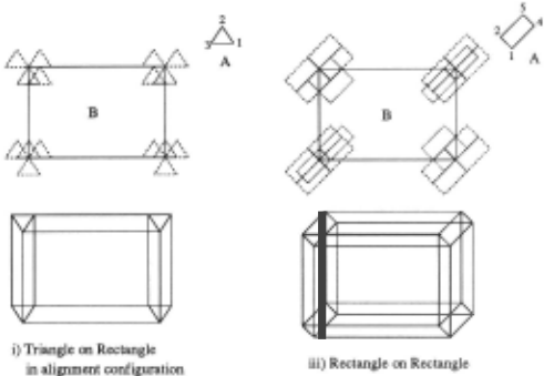
Figure 6: The CF maps for the configurations (i) and (iii) in the previous figure. The upper part shows the two faces in contact positions; the lower part the CF map. The regions correspond to the contact formations where two d.o.f.'s are available which maintain the contact, the lines where only one is available and so on.
Note that this algorithm is used to find the slices cor responding to purely translational motion such as (i) in fig 5, but also for a representative instance of a quali tatively invariant zone, such as all rotations about the alignment edge, for which the CF map in fig 6(iii) is a boundary slice.
Complexity: Let n and m be the total number of faces in A and B. The number of alignment relations depends on the number of faces that are 1-manifold or above (Ver tices sliding on an object reproduce that object itself) , a number that is bounded by n. In general, there are O(nm) candidate alignment configurations. For each of these, the algorithm above requires O(nm) time in com puting the translated objects, and O(k + nmlog(nm)) time in evaluating the intersections for 2-faces, where k is the number of actual intersections (For 3D. faces , whatever that may mean, it would be O(n 2 m 2 )). Thus , for objects upto E 3 the complexity of the algorithm for finding all CF maps for all the slices is O(n 2 m 2 log(mn)) if k is less than nm log( nm). If n = max( n, m), then this is O(n 4 logn).
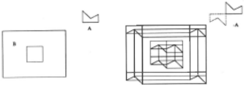
There are several other aspects of this algorithm. If one of the faces is non-convex, or even has a hole, the algorithm still determines the CF maps correctly, since it is based on a linear sweep between the edges, which lo cally results in the correct translational boundary (Fig. 7). A side benefit of this computation is that it makes it simple (an O(nm) planar sweep postprocessing) , to compute the C-spaces for polyhedral obstacles, a prob lem for which solutions appear to be known only in the convex cases [16]. A simple strategy like plane-sweep can be used to determine the boundary of the map which is then the C-space of the objects in question. Note that taking just the convex hull , as suggested earlier, wi~l n?t give the C-space. A traversal .t~rough the f~ce-hst m this map yields the CF connectivity graph as m figure 8 which ca~ be used for assembly. In the following section, we integrate the above methodology to provide a search space for Fine Motion Planning.
m "
Figure 7: A CF map for a non-convex peg on a rectangle with hole.
5 The 2-Body Problem
The assembly problem consists of taking a set of bodies that were initially separated into contact. The principal difference with path planning is that there are multiple bodies (although they are often considered monotoni cally in subassemblies), and that the initial configuration is not fixed . Other differences include the occasional need to find space to temporarily hold subassemblies. The part of this problem that has received the maxi mum attention is the sequence planning problem, and the part that has received the least attention, undoubt edly because of its intrinsic difficulty, is relating it to the geometry. In the following , we present an algorithm for obtaining the contact motions of two objects, or what we call the 2-body problem. This constitutes a single link in an AND/OR or other "high-level" assembly graph. To our knowledge this is the first model that provides a reasonable process for mapping these connectivity links directly to the geometries of the objects. We now give an algorithm for assembly by searching through the contact formations .
Algorithm
- Construct the contact formation map assuming full domain degrees of freedom (i.e. no limit angles etc) . Also, obtain the C-space in this process.
- Adding the constraints, consider the surfaces caused by the constraints. These surfaces do not have any internal CF features , since the entire surface corre sponds to a stop position. In other words, these surfaces can delete some CF maps that arise in inaccessible re gions, but cannot add any new CFs.
- For each CF identify the configuration patch (CP) corresponding to it on the C-space. If this region is not connected (e.g. for null CF) then split the separate con nected components, and label these as separate sub-CFs.
- Scan all the CPs and connect adjacent CF's corre sponding to adjacent regions on the slice by undirected edges.
This returns a CF graph indicating connections in the Contact Formation space and provides a very basic search space for further queries and operations. Each region in this space can be directly related to boundary features on the object. All standard AI methodologies such as learning based on densities , incremental defini tion etc. can be used on this graph to reduce the search complexity. It may be noted that all those regions which formed the boundary of the original C-space are part of the boundary of the constrained C-space also, except that they have added internal features on these indicat ing the richness of the CF structure in it .
The CF graph is useful in solving a variety of spatial problems. To answer the query about the cube rolling down a plane, originally posed in [1], we can move from slice to slice as the cube rotates, to obtain directly the sequence of vertex edge and face contacts as they are made and broken. To investil!iate the kinematic problem posed by Forbus et al in [10J, where one would like to say how two wheels "one with a bump on it and the other with a notch carved out of it" will travel , one can build the CF map, which provide a discretization for the Configuration Space methods proposed earlier. As for assembly, we illustrate the applicability of the CF map by outlining the solution to the peg insertion problem posed (Fig. 4) . The graph resulting from the CF map is shown in Fig. 8, and the set of CFs is listed below (the edge between vertices i and j is represented by ij).
Another aspect of the CF graph is that each constraint reveals the degrees of freedom that exist in maintaining that constraint . e.g in fig. 6(i), the slice is fully con strained in rotation, and hence the vertices in the graphs represent zero degrees offreedom (annotated as CF 0 's). The edges in this diagram, as well as the vertices in (iii) which permit a rotation, permit one degree of freedom and constitute CFI's. The intersection process results in a depletion of freedom; the intersection of C Fr and C F9 results in a CF$, where s = d-(d-r)-(d-q) = r+q-d. This is an important notion in designing assemblies to have certain d.o.f's and reveals where on the surface to place constraining grooves or other similar questions.
Example
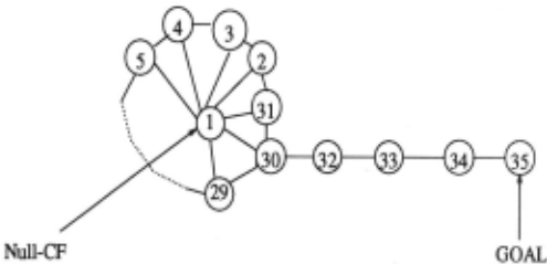
| 1. Null 3. ( c, 12), (b, 12), (be, 12) 5. (c, 12), (1, be), (be, 12) 7. (1, cd), (c, 18), (18, cd) 9. ( c, 1~ ( d, 18), ( cd, 18) 11. (8, cd), (d, .!!), (cd, 18) 13. (d, 78), (8, ad), (78, ad) 15. (a,78),(d,~,(78,~ 17. (a, 78), (7, ad), (78, ad) 19. (a, 67), (7, ab), (67, ab) 21. (a, 67), (b, 67), (67, ab) 23. (6, ab), (b, 67), (67, ab) 25. (b, 56), (6, be), (56, be) 27. (b, 56), (c, 56), (56 , be) 29. (5 , be), (c, 56), (56, be) 31. (b, 12), (2, be), (be, 12) 33. (a, 2), ( d, 5), (b, 32), (c, 54), ( cd, 54), ( ab, 32) 35. (b, 3), (c,4), (be, 34), (a, 32), (d, 54), (cd, 54), (ab , 32) | 2. (c, 2), (b, 12), (be, 12) 4. (b, 1), (c, 12), (be, 12) 6. (c, 1) 8. (1, d), (c, 18), (18, cd) 10. ( c, 8), ( d, 18), ( cd, 18) 12. (d, 8) 14. (8, a), (d, 78), (78, ad) 16. (7, d), (a, 78), (78, ad) 18. (7, a) 20. (7, b), (a, 67), (67, ab) 22. (a, 6), (b, 67), (67, ab) 24. (b, 6) 26. (c, 6), (b, 56), (56, be) 28. (b, 5), (c, 56), (56, be) 30. ( c, 5), (b, 2) 32. (b, 32), (c, 54), (cd, 54), (ab, 34.( a, 32), (b, 32), ( c, 54), (d, 54), S(cd, 54), (ab, 32) |
We see from the figure a number of paths exist between the START and the GOAL positions eg. 1,30,32,33,34,35 and 1,3,2,31,30,32,33,34,35 etc. These correspond to al ternate mechanisms for executing the assembly. Unlike other assembly planning systems, the CF map allows one to distinguish between these choices not only based on connectivity but also on other functional issues such as landmark configurations, the existence of similar error configurations, etc.
6 Conclusion
This work provides a novel methodology for spatial ob jects in 2D and 3D, to derive qualitative maps of rela tive motions. The discretization claims to be qualitative since it is compact, the entire set is determinable based on functional features of the domain, and the knowledge maintained provides direct explanation power since the set of surface features in contact are critical to explaining many tasks. As illustrated in our focus domain involv ing parts assembly, the applications of this procedure can provide rich dividends in a number of problem areas. In a sense this work is a synthesis of radically different lines of thought from robotics, qualitative reasoning, assem bly planning, and vision, but the end result sufficiently different from the methodologies in any of these to be viewed as a new tool in the arsenal of qualitative reason ing.
@inproceedings{ijcai1995p119,
  title     = {A Qualitative Discretization for Two-Body Contacts},
  author    = {Mukerjee, Amitabha and Agarwal, Manish and Bhatia, Praveen},
  booktitle = {Proceedings of the Fourteenth International Joint Conference on
               Artificial Intelligence, {IJCAI-95}},
  publisher = {International Joint Conferences on Artificial Intelligence},
  editor    = {Chris S. Mellish},
  pages     = {915--922},
  year      = {1995},
  note      = {Knowledge Representation},
  url       = {https://ijcai.org/proceedings/1995/119},
}
TY - CPAPER TI - A Qualitative Discretization for Two-Body Contacts AU - Mukerjee, Amitabha AU - Agarwal, Manish AU - Bhatia, Praveen T2 - Proceedings of the Fourteenth International Joint Conference on Artificial Intelligence, IJCAI-95 PB - International Joint Conferences on Artificial Intelligence PY - 1995 SP - 915 EP - 922 UR - https://ijcai.org/proceedings/1995/119 ER -Copied
Machine-readable versions of this paper, for tools and AI agents:





