Diagnosis Process Dynamics: Holding the Diagnostic Trackhound in Leash

1. Introduction

In recent years reasoning about structure and functioo of physical systems for the purpose of diagnosis has seen a dra­ matic increase in activities. A considerable set of new excit­ ing results have emerged from these:

• modelling issues such as representation and use of tem­ poral aspects [Hamscher 91], models of different granular­ ity, relations between models [Struss 92], and multiple compooent modes [de Kleer, Williams 89]
• diagnostic inference patterns, e.g. alibis [Raiman 89], physical negation [Struss, Dressler 89] and physical impos­ sibility [Friedrich et al. 90]. integration of abduction e.g. [Console, Torasso 90], use of non-intermittency [Raiman et al. 91], and
• inferential power [de Kleer 91].

Nevertheless, a main obstacle for building large diagnostic systems remains. How can we control when to use which inference pattern oc representation ?

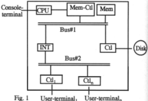
Consider the example from [Davis 82]. A computer is appar­ ently working fine when viewed from the console terminal. The hardware powers up, the operating system loads and runs. The user terminals appear functional, but nothing hap­ pens when we type something.

Supplied with a very coarse model, a diagnosis system like GDE [de Kleer, Williams 87] can identify the computer as the most probable suspect. At this point the best diagnostic action is a structural decomposition. But why this one instead of a switch in behavioral model granularity for one of the termi­ nals for example ?

Structural decomposition moves us to another world illus­ trated in fig. 1. If disk, cootroller, bus#l, memory, memory control or cpu were malfunctioning, the operating system would not be running. Supplied with the diagnostic hypothe­ ses that fault modes for these compooents are complete, GDE+

Oskar Dressler · Siemens AG MUnchen, Germany dressler@zfe.siemens.de

[Struss, Dressler 89] can exonerate all of them. But why choose the diagnostic action of adopting fault mode completeness for exactly these components instead of e.g. a structural decom· position of a non-suspect component ?

In only two diagnostic steps the available diagnosis machin­ ery could pin down two highly suspicious components, namely the bus interface INT and Bus#2, because we have chosen the right diagnostic actions by hand. A few more steps lead to a bent spring-loaded connector between a board and a ?ack:plane slot. Coosider the enormous reduction in complex· 1ty ! The key to cootrolling inference in large diagnostic pr<» lems is the ability to choose between diagnostic actions and know when to do it. ·

Carefully choosing the right technique at the right time would allow minimizing the overall cost of model simulation, mea· ~ent selection, probing etc. But the conventional diagno­ SiS loop of predicting behavior by simulating (component) models, detecting discrepancies, e.g. between observed and predicted values, generating diagnoses and, finally, discrimi· nating among the most plausible diagnoses by additiooal measll(ements is inadequate for at least two reasons:

• In general, there is a lot more reasoning that can be done before the agent needs to go probing. It can e.g. switch to structurally or behaviocally more refined models oc adopt or drop diagnostic hypotheses such as fault model com· pleteness, preference for explaining diagnoses or about the nature of faults, e.g. non-intermittency.
• Even though we have seen a fundamental breakthrough in inferential power [de Kleer 91] the agent cannot afford to run all component models etc.

Therefore, we need a framework for deciding when to take which action, i.e. when to switch a model, take a measure­ ment, drop or adopt a diagnostic hypothesis. etc.

Approach and Outline

Changing hypotheses means changing the agent's belief state. Consequently we treat the coo.trol problem as a belief revision problem. A belief state change is triggered by either the cur­ rent state not allowing for the generation of plausible diag­ noses or the existence of a more preferred "neighbor". The guiding principle for revision is informational economy [GHrdenfors 88] which we independently motivate for diagnos­ tic contexts. Acting as a kind of law of inertia for diagnostic processes it requests that changes to the current working hypotheses have to be minimal and provides the basic candidates for revision. A belief revision operator defmed in terms of these candidates automatically eliminates useless changes due to logical relations e.g. between component models or component modes. From the remaining changes the most pre­ ferred is chosen drawing on general knowledge aboot assess­ ing diagnostic belief states qualitatively. Since every diagnostic action can be identified as a change of working hypotheses selecting the best next belief state amounts to selecting the best next diagnostic action.

Section 2 shows how we represent mode and model assump­ tions in relation to models. Introducing the notion of preferred diagnosis we specify our representation of an agent's belief state. In section 3 we turn to the dynamics of diagnostic belief state changes and identify two forms of non-monotonicity involved. Section 4 and 5 provide the technical details concerning informational economy. our belief revision operator. computation of basic candidates for revisions and selecting the best next belief state for the diagnosis process.

2. Diagnostic Belief States

A model-based diagnostic agent is supplied with a system description SD and a set of observations Obs. Often we refer to SD U Obs as the background theory T. Two basic insights help structure SD. Consider the model of the computer in the example. First, at the beginning we only need a very coarse model using qualitative input/output values like 'looks fine' or 'looks bad'. In later stages of the diagnosis process more detailed models may be required. Second, the computer might work in different good and fault modes that need to be repre­ sented as different models. Combining both requirements we represent model chunks for component c as formulae of the I form modg 1\ mode(c) /\. ... ~ ....

I where mode(c) identifies the component mode and modg the model granularity. For instance, the implication

fme/bad-level/\ ok(computer) 1\ input=looks-fme

~ output=looks-fme

describes the computer at a coarse level for its ok mode.

A focused ATMS ([Dressler-Farquhar 90], [de Kleer 91]) allows using the model granularity and mode preconditions for con­ trol purposes. Predictions will oo.ly be made when the precon­ ditions are activated during the diagnosis process. To control the activation the agent maintains a set of working hypotheses w. This may include model granularity and mode assumptions as well as diagnostic hypotheses, e.g. aboot the nature of faults. These "precondition" assumptions and logical relations between them are known to the diagnostic agent as part of SD but no predictions are made unless they are selected. Once made, however, predictions are cached in the ATMS.

Assigning modes of behavior to the e<mponents of a device is a central task of the agent. Mode assignments must be consistent with the observations and the worlcing hypotheses cur­ rently held. Worlcing hypotheses are taken from the set WHP containing among others model granularity assumptions and diagnostic hypotheses. Subsets of WHP are called worlds. We represent worlds w by their "w-closure", i.e. WHP n Cn ( w U 1). \Yhere Cn(A) := {a I A derives a}.

Def. 2.1 : Let modes (C) denote the modes of a component C. A mode assignment n E modes (C1) x ... x modes (Cn) (denoted{ .. Dl_j(Ci) .. }) is a diagnosis under hypotheses w iff SD u Obs u w u n is satisfiable.

Not all diagnoses are equally plausible. One reason is that dif­ ferent mode assignments to an individual component may have different plausibility. e.g. ok modes are preferred over fault modes. We assume that a partial order :<!:for the modes of a component is given. If needed, this order may depend on a corresponding working hypothesis and thus may be subject to later revisions. Preference relations among modes induce a preference relation among diagnoses: let n = { .. Dlj(Ci) .. } and n· = { .. 11\:(~) .. } be two diagnoses in world w. Then n :<!: n· iff v i=l. .. .n: Dl_j(Ci) :<!: m' k(Ci).

Def. 2.2 : A diagnosis n is a preferred diagnosis under working hypotheses w iff no diagnosis under w is strictly preferred over it v n·: n· :<!: n => n· = n

Example: Let the user terminals have three modes, ok > fm1 > fm2· and the computer have two modes, ok > fm. If all com­ binations of fault models are consistent with the observations, then {ok(console), fm(computer), ok(term#l), ... , ok(term#n)} and {ok(console), ok(computer), fm 1 (term#l) , , fmj(term#n)} are preferred diagnoses, but {ok(console), ok(computer),fmiterm#l ), ... ,fm1(term#n)} is not.

In what follows we omit ok modes, e.g. {fm(e<mputer)} denotes the first preferred diagnosis from above. We encode component modes as normal defaults with prerequisites [Reiter 80] ... A -mi(C) A .· : Dl_j(C) I mi_C) denotes the default for the j-th mode of component C. This guarantees that a mode Dl_j(C) will be considered only when the more preferred modes .. ~(C) .. have been refuted. These defaults can be encoded in a non-monotonic ATMS. This NM-ATMS com­ putes minimal consistent extension bases, MinExtBases (D. w u n. that are in one-to-one correspondence with the exten­ sions of the default theory .l=(D. w u n and hence preferred diagnoses.

Theorem 2.1 : n is a preferred diagnosis under hypotheses w iff 3 B E MinExtBases (D. w u T): TI!;;;;; Cn(w u B u n.

The belief state comprises predictions made from SD U Obs. They are indexed by the underlying mode and model granu­ larity assumptions. If w u T has no consistent extensioo, then w is said to be incoherent. It is the incomplete set of observa­ tions about the artifact and the inconsistencies discovered that give rise to multiple extensions, and hence multiple plausible diagnoses. See [Dressler, Struss 92] for details.

3. Diagnostic Belief State Change

Diagnosis is a sequential process. During this process the set of plausible candidates for diagnosis may expand as well as shrink depending on choices taken by the diagnostic agent. Each choice plays the role of a working hypothesis that may be retracted later on, only to be re-adopted under some future circumstances. In the first step of the example there are two preferred diagnoses, namely {fm(computer)} and {fm(term# 1). .. fm ( term#n)}. We zoom into the computer's structure. This leads to preferred diagnoses such as {fm( bus#2)}, i.e. we expand the set of preferred diagnoses. Imagine that further observations lead us to conclude that everything is ok with the computer. All of the new diagnoses are refuted. Then we shrink the set of preferred diagnoses.

There are two forms of non-monotonicity involved. Logical non-monotonicity occurs when an agent generates expecta­ tions about plausible inferences based on its current incom­ plete belief state. Temporal non-monotonicity occurs when an agent changes its belief state by dropping some beliefs while possibly assimilating others. It is crucial to understand that belief state changes are often motivated by reasons beyond logic. For example, an agent may want to change its belief state not only because it has become inconsistent but because it simply prefers another, e.g. when the number of preferred diagnoses differs by an order of magnitude.

Both, temporal and logical non-monotonicity are needed for a natural formalization of the behavioc of diagnostic agents. The rest of the paper deals with temporal non-monotonicity. We discuss two scenarios separately. They correspond to the two reasons for triggering a belief state change:

• the selected set of working hypotheses does not allow for the generation of diagnoses
• there is a more preferred "neighbor" wocld

4. Revising Incoherent Belief States

4.1 Plausible Candidates for the Next Belief State

We start with the former scenario, i.e. A= (D, SD U Obs U w) has no extension. We consider the potential move from a set of working hypotheses w 1 to a set w 2 . In a different termi­ nology we could say that all propositions but the wocking hypotheses are protected formulas. Some of the selected working hypotheses are going out, some others are about to become in. The union of these tells us how much is changed in terms of working hypotheses when moving from w 1 to w2. Since we represent worlds by their deductive closure, the def­ inition is less syntactical than it appears. Logical connections between working hypotheses are reflected, e.g. the "at most one fault" assumption implies "at most two faults" etc. Fur­ thermore, we include integrity constraints on woclds requiring for instance that (at least) one model granularity assumption is activated for every component.

Def. 4.1: diff (w1,w2) := (w1 \ w2) u (wz \ wl)

When a selected world is incoherent, i.e. has no consistent extension, the diagnostic agent has to decide whether there is another world allowing for the generation of diagnoses. It has to make a choice between the possible moves, but should not select an arbitrary one. There are at least two reasons: First, the primary sources of diagnostic information are the sets of assumptions underlying a contradiction (conflicts). At least one of the components is not wocking in the specified mode or a working hypothesis is violated. Therefoce, on the one hand we want to keep the diagnostic agent focused on these assumption sets. On the other hand there is the need to change the working hypotheses. Allowing only minimal changes of the selected set of working hypotheses minimizes the risk of losing conflicts. This is the main argument for the principle of informational economy in diagnostic contexts. There is a sec­ ond, computational one. Allowing non-minimal changes might shift already cached intermediate results out of focus. This is especially the case when using a focused A TMS. Therefore, exploring totally new foci is more expensive than explocing partially new ones. Possible moves are collected in the set 'revisions' below. The definition is given in terms ci preferred diagnoses and minimal set difference of source 8lld target world.

Def. 4.2: Let w be a world. Revisions (w) :=

{ v E worlds I 3 preferred diagnosis under v and diff(w,v) is minimal wrt. set inclusion}

Whether a diagnostic action is useful only becomes clear when behavioc prediction based on the selected hypotheses is done and the agent reaches a new belief state after generatina diagnoses. But simulating models for the sole purpose ci deciding which action to choose already performs those can· potations most of which we want to save. Hence, a limited lookahead is needed. The effects of a diagnostic action are essentially determined by the set of selected hypotheses resulting from the action. A diagnostic action moves the agent from its current world w 1 to a target world w2. And of course, the target world should allow for the generation of diagnoses, i.e. be coherent. Since we cannot invoke behavioc predictioo for deciding whether w2 is indeed coherent, we use an approx· imation. We only use the inferences cached in the ATMS fer making the decision. This·means that the decision whether a target world is coherent is made on the basis of already simu· lated models only. This adequately reflects our view that the agent uses its limited knowledge that characterizes the current diagnostic situation.

4.2 Revision Operator

The set revisions(w) is but a set of plausible "neighboring" worlds. The diagnostic agent still has a choice as to which of these worlds it wants to enter. The function 41 selects it.

Def. 4.3 : Let 41 be a selection function and w E worlds. The revision operator rev-op is rev-op(w) := 41 (revisions (w)).

4.2.1 Exploiting Logical Relations

The operatoc is surprisingly powerful in diagnostic contexts. By definition it avoids target worlds where no diagnoses exist. This eliminates almost all useless diagnostic actions the agent could perform otherwise. We consider two examples. The ftrst one is structural decomposition. It shows how logi· cal relations between component modes are automatically exploited by the revision process. The second is the use ci simplifying assumptions which stands for the class of logical relations between component models.

Example: H the computer's subcomponents are ok. the can· puter should be wocking correctly. In order to provide a han· dle for control and to reflect implicit assumptions like tbe above, we include the model granularity assumption modg· Csub in the implicationmodg-csub 1\ ok(cpu) ... 1\ ok(disk)-+ ok (computer)

which is part of the system description SD. Structural decool· position of the computer model means adding modg-<;w, to the current world w. H, however, no preferred diagnosis exists, then, so the following lemma tells us, no superset of w has one either. Hence, adding modg-c 8 ub is not a choice takm by the revision operator in our example.

Lemma 4.1 : For all w' ;;;2 w: if there is no preferred diagnosis under w then there is no preferred diagnosis under w'.

Example: A (component) model m' is a simplification of another model m, when values entailed by m' are also entailed by m and a simplifying assumption o, [Struss 92]. Let M and M' be the associated model granularity assumptions. Then M " o ~ M'. Simplified models are often much easier to simu­ late than more detailed ones. Therefore an agent starts with the simplified model, i.e. M' E w. In case no preferred diag­ noses under w exist, due to the last lemma, activating the detailed model and the simplifying assumption, i.e. o, M E w. does not lead to diagnoses since they imply M'. The revision operator will not do that. Deactivating o, i.e. o It w, M E w, could help if there are no other causes for the non-existence of diagnoses.

4.2.2 Preferences between Worlds

Exploiting logical relations avoids useless actions such as refining a non-suspect component. But there is more diagnos­ tic knowledge available. The selection function cjl need not be that blind when selecting an element from revisions(w).lf e.g. the number of preferred diagnoses in a world w1 is an order of magnitude greater than in w2 then prefer world w2. In [B~t­ tcher 91] a variety of such examples are discussed.

Example: Physical negation concludes, that when all fault modes of a component are known and have been refuted, the component must be ok. E.g.

-,£m(cpu) A fault-modes-complete(cpu) ~ ok(cpu)

If SD U Obs U w U {fm(cpu)} is not satisfiable, then adopting fault-modes-complete(cpu) leads to ok(cpu). Hence all preferred diagnoses under w' ;;;;;! w assigning a fault mode to the cpu are eliminated. Nevertheless, as long as the fault mode has not been refuted, the described effect will not take place. In this case the operator has no preference for adopting fault-modes-complete(cpu) because the set of preferred diag­ noses remains the same.

The last example gives a flavor of the preferences that can guide the selection of worlds. It is also in order to make use of criteria like e.g. probabilities for the applicability of working hypotheses. when they are available. For the selection of diagnostic actions in general, however, we can only e~t to have a diction~f p~preferences DPP ={DPPi I i E l...n, DPPi !;;;;; 2 x 2 } . Ideally, one would want to aggregate a global preference order from DPP in order to allow for a rational choice by the selection function cjl. This, however, is impossible given the results reported in [Doyle 91]. It is shown that no aggregation policy exists that could aggregate a collection of partial preferences, e.g. DPP, into a global order satisfying fairly mild restrictions. The order below therefore is defmed with the goal that the diagnostic agent can use obvious preferences when available.

Def. 4.4 : (Aggregation Policy)

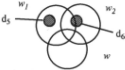
Let w, w 1 , w 2 be worlds. w1 ~w w2 iff [(3k 3(d 1 ,d 2 ) E DPP~c: d1 !;;;;; w1 "d2 !;;;;; w2) " ~(3j=lf=k 3(d3,d4) E DPPj: d3 !;;;;; w2 A d4 !;;;;; w1)] V3I3 (d5.~ E DPPi: d5 !;;;;; w1 \wA~!;;;;; w2 \w

It prefers a state w 1 over w2 when no opposite preferences are known (fust disjunct). Nevertheless, large worlds tend to be ordered ~multiple ways by different DPPi. Therefore, w1 and w 2 are likely not to be ordered by the first disjunct because their overlaps with the current world w may already contain t~o opposite preferences. A preference, however, may be jus­ tified because of the new hypotheses added in the candidate v.:orld~ w1 and w2. ~s is achieved by the second disjunct. Flg.2 Illustrates the situation.

The selection ~ction cjl for the revision operator rev-op chooses a maxmally preferred world in revisions (w) with respect to the aggregated order ~w·

We can encode a wide range of preferences. In a moment we shall list some common preferences that apply to large classes of diagnosis applications. Most of these preferences can be derived from the fact that we are doing diagnosis of an artifact that worked before and was not e.g. the target of a bomb ~ttack. Therefore, one can assume that a small percentage of Its components are defective. Hence. it makes sense to prefer actions that aim at proving correctness of suspected compo­ nents, e.g. via physical negation, or to delay further elabora­ tion on suspects, e.g. via structural refmement, until they are clearly identified. In general, preferences may depend on the current world w and its set of preferred diagnoses diag(w ). Let COM~ denote the. set of all components and moderr(c) be

the behav10r mode assigned to component c by diagnosis n

Pl: Structural Refinement

S~ppose. our diagnostic agent currently operates on the i-th hierarchic layer of some component c and considers a struc­ tural .refinement ~ a possible move. This is reflected by a working hypothesis for the current layer of c, say ~(c), in the current world and hi+ 1 (c) in a coherent neighbor world. We do structural refinement only, if the component is identified uniquely as defective:

P2: Behavioral Refinement

If a model m(c) (possibly under some working hypothesis) makes s~ctly stronger predictions than another model m'(c), then refutmg the weaker one also refutes the stronger ([Struss 92]). Therefore, when multiple models for the same behav­ i?ral mode are available, we prefer simpler models when pos­ sible. If we want to discriminate between diagnoses, however, we try to refute some of them. This can be done by making stronger predictions, e.g. switching to stronger models for the behavioral modes occurring in the diagnoses.

if3 Il1,Il2 E diag(w) 3 c E COMPS: modem (c) *modem( c) then { m(c) } >n { m'(c) } for all other components: { m '(c) } >n { m(c) }

P3: Physical Negation

We avoid assigning the unknown behavioral mode to a com­ ponent with known fault modes by physical negation:

if 3 IT E diag(w) : moderr(c) =unknown( c) 1\ 3 mode(c) *unknown( c): mode(c) ~ -ok(c) then {fault-modes-complete(c)} >rJ {} else {} >p3 {fault-modes-complete(c)}

P4: N-Fault Assumption

Simple diagnoses in terms of the number of broken compo­ nents are preferred:

if i <j ~ #COMPS then { at-most-i-faults} >p4 { at-most-j-faults}

PS: Non-Intermittency

Presuming non-intermittency for a behavioral mode allows the agent to predict identical outputs of a component at time ti given the same inputs as at some other time~ ([Raiman et. a!. 91]). As long as feasible, we assume non-intermittent modes: 'if c E COMPS 'i/m E modes( c): {non-intermittent(m)} >p5 {}

P6: Further Measurements

When the current world is the most preferred one. the agent longs for more external information. It makes sense to take additional probes. if this discriminates between preferred diagnoses. Finding optimal discriminating points is a function of the measurement proposer as in [de Kleer, Williams 87]. If, however, no additional measurement can discriminate between the preferred diagnoses, then a measurement can at best refute them all. In this case the agent prefers to make any other available move instead of doing random probes.

if no-more-discriminating-measurements ( w)

then 'if a E WHP: {a} >p6 {}else {} >p6 {a} In expressing this preference we have implicitly assumed that probes are associated with some non-negligible costs. This is not the general case. In many applications the measurement proposer can act as an intelligent, situation dependent filter that selects from anyway available observations. Therefore, it may be advisable to do more probes. i.e. gather more evi­ dence before investing all the effort to find plausible interpre­ tations of an incompletely described situation:

if more-measurements (w) then 'if a E WHP: {} >P6· {a} else {a} >p6· {}

All of these preferences can be further elaborated. Often they can be tuned by exploiting application characteristics, e.g. if a component is likely to fail in some unpredictable way. then we better avoid applying the physical negation rule. For another example consider P2, behavioral refmement. If we have tried a stronger model for a component upon which two different diagnoses disagree, but none of them is refuted, then we can make even stronger predictions by switching to more detailed models for more of the other components.

4.3 Computing Revisions

The key insight to computing revisions(w) is the following observation: given the working hypotheses diff (w1, w2) that are either going in or going out when changing from w 1 to w2, and the current world w 1· we can determine the target world w2: diff (w 1· diff (w 1· w2)) = w2

This allows monotonically enumerating potential diffs breadth first starting from the empty set. Since we are inter­ ested only in minimal diff's that satisfy certain conditions. we avoid testing arbitrary target worlds.

com pule-revisions( w)

vars: agenda:= { {} }, coherent-diffs, d, diff loop until empty( agenda) do d:= pop( agenda) loop for h in working-hypotheses do diff: = {h} U d ; target:= diff(w, diff); if subsumed (diff, coherent-diffs) then nothing else if coherent (target) then add-and-minimize (target. coherent-diffs) else push (diff. agenda) return-values:

loop for cdiff in coherent-diffs collect diff (w. cdiff)

We perform a breadth first seareh in the lattice of sets of working hypotheses. i.e. the search order for diff is { } .

{hd ..... {~}. {h1· h2 }. .. . If it leads to a coherent world, we update a set of minimal diffs, coherent-diffs. Otherwise we push diff on the agenda, i.e. we expand it the next time through the loop. We stop when it is subsumed.

Usually the algorithm stops after just two top level iteratioos since a multiple change of working hypotheses is seldom required. But the main effort for computing revisions(w) is hidden in the predicate coherent. It requires that MinExtBases be computed ([Dressler 90]). This. however, is no additional overhead. The NM-ATMS computes MinExtBasesanyway foc the generation of preferred diagnoses (theorem 2.1).

5. Revising Coherent Belief States

!f the current world is incoherent a belief state change is inev· Itable. But there may be other reasons. ·

Example: If there is a preferred diagnosis assigning a fault to the computer, it may make sense to refine its structure since -,ok(computer) A modg-csub--+ ook(cpu) v .... v-,ok(disk) ~ thi~ ca~ the revision operator could select modg-csub for mcluswn m w. Because of suspecting the computer the agent expands the substructure thereby generating a multitude d preferred diagnoses. Now, if a technician measures the com· puter's output towards the terminals and finds that it is ok, then the computer is no longer suspect. Moving back to the black box level of the computer, i.e. dropping the assumption modg-csub would result in significantly fewer preferred diag· noses. Therefore the agent prefers this world without being forced by logical reasons.

We still accept the principle of informational economy. Diag· nostic actions should not jump to arbitrary target worlds. But in contrast to the situation discussed in section 4 the current world is coherent. There is at least one preferred diagnosis. The agent may take the opportunity to strengthen its positioo by adopting stronger working hypotheses that, when added, still allow for the generation of diagnoses. Consider foc ~stance the initial situation when the diagnosis process has Just been started. The empty world is coherent (modulo poten· tially violated integrity constraints) since no prediction wPJ performed, hence no contradictions detected so far. The agent may now adopt working hypotheses. We allow it to iterate choosing "neighbor" worlds without interleaving prediction. This means that the agent can choose a maximally preferred world from all worlds that can be reached from the current world without traversing an incoherent one. Of course, it may also choose the current world because it is coherent. The selection process then is roughly similar to the one discussed in the last section. The main difference is that the current world may be a possible candidate for a (non-) move.

select-next-world (w) var: next-world if incoherent ( w) then return <1> (compute-revisions (w)) else loop for next-world := <1> (compute-revisions (w) U {w}) until w =next-world dow :=next-world fmally return next-world

6. The Example Revisited

Initially, there would be two preferred diagnoses, {fm(com­ puter)} and {fm(term#l), ... , fm(term#n)}. but preference P4

leads to the selection of the initial world w 0 ={at-most-1-fault}

which avoids the second diagnosis. The only diagnosis under w0 uniquely determines the computer as defective, hence Pl selects

w 1 = { at-most-1-fault, modg-c sub( computer)} .

Now the internal structure of the computer becomes visible to the diagnosis agent. Because the path from the console termi­ nal to the disk is functional (the operating system runs !), all known fault modes for components along that path are refuted (while those for other components are consistent). Conse­ quently, they are assigned the unknown mode in all preferred diagnoses generated under w 1 . For exactly these components P3 selects the fault-modes-complete hypotheses, fmc.

w2 = { at-most-1-fault, modg-c sub (computer), fmc(cpu),fmc(mem-ctl),fmc(mem),fmc(bus#1), fmc(ctl),fmc(disk)}.

The preferred diagnoses are {fm(int)} and {fm(bus#2)}.

The diagnosis process as described in [Davis 82] proceeds by taking further actions such as structurally refining bus#2, doing a few more probes, switching between alternate models etc. and fmally settles on a bent spring-loaded connector.

Provided we had available a diagnosis system that integrated all the necessary diagnosis techniques e.g. alibis, physical negation, physical impossibility, use of non-intermittency and multiple models, generation of test-vectors, probe selection and an appropriate set of preferences, it should now be possi­ ble to re-conStruct the entire process put forward by Davis as a challenge to the AI -community in 1981.

7. Implementation

We have built a system called 'Magellan oi that uses the described revision operator. It is applied to the diagnosis of ballast tank systems where the control of multiple, qualitative and quantitative models is crucial [Dressler et. al. 93].

8. Related Work

[Struss 89] provides a framework for representing diagnostic hypotheses, a necessary precondition for reasoning with them. Few have followed this avenue since then. An excep­ tion is [Nejdl91] where the notion of 'plausible world' is intro­ duced. A set of such worlds represents a belief state. In contrast to our approach Nejdl's worlds resemble models of the diagnostic situation, i.e. a valid interpretation rather than a set of working hypotheses. Therefore, Nejdl in essence com­ pares different diagnoses while we compare different worlds and thereby sets of diagnoses.

The problem of guiding the diagnostic process is an instance of the more general belief revision problem. This is an active research area within AI, e.g. [Doyle 91], that should have a major impact on diagnosis in the future. Notions, however, like e.g. epistemic entrenchment are important, but not strong enough to provide guidelines for diagnostic processes.

9. Conclusion

We have presented a framework for organizing diagnosis processes that exploits and adapts belief revision for diagnostic purposes. Informational economy is the basis for determining candidates for belief state changes of diagnostic agents. Working hypotheses as used in diagnosis systems are the atomic units for building belief bases. Additional diagnostic information allow the agents to make a rational choice not only in terms of an emerging overall belief revision theory but also in terms of preferences specific for diagnosis.

I. Femi{o de Magalhi{es (1480-1521), portuguese sailor

Acknowledgments

Hartmut Freitag, Michael Montag, Peter Struss, Monika Pfau, Wolfgang Nejdl, Thomas Guckenbiehl, Claudia Johnson and Liibbe Onken commented on earlier drafts. This work was supported by BMFT, project BEHAVIOR, ITW 9001 A9.