
TDIS : an Algebraic Formalization
Proceedings of the Thirteenth International Joint Conference on Artificial Intelligence. Machine Learning. Pages 1008-1014.
© 1993 International Joint Conferences on Artificial Intelligence
Abstract
In the light of the success of Top-Down Induction Systems (TDIS), the problems to be addressed concern the structure of descriptions and the exploration of strategies. This paper introduces a formal model to describe TDIS, based on the use of lattice theory and, more precisely, on the use of a Galois connection. One of the advantages of this formalization is that it justifies the extensive use of attribute-value representation in the case of classical TDIS and generalizes this representation to products of hierarchical posets. In addition, given that there are many different learning strategies for TDIS, this formal model shows the limitations of classical strategies and offers a general framework in which many other strategies can be expressed.
- I967]., Lattice theory, Third Edition, American Mathematical Society, Providence, RI I967.
- Clark and Niblett I987] ''The CN2 Induction Algorithm", Machine Learning, 3, p. 26I-283.
- Gams I989] "New Measurements Highlight the Importance of Redundant Knowledge", EWSL-89, Glasgow, United- Kingdown, I989.
- I987], "CHARADE: a rule system learning system",IJCAI 87, Miian,ltaly, I987. IJCAI
- I992] "An algebraic fornnlization of CHARADE", LAFORIA, Internal report, November I992. [Ganascia eta/., I993], "Integrating Models of Knowledge and Machine Learning", to appear in ECML-93, April I993, Vienna, Austria.
- I978] General Lattice Theory, Academic Press, New-York, I978.
- I983] "Learning efficient classification procedures", Machine Learning: an artificial intelligence approach, Michalski, Carbonell & Mitchell (eds .), Morgan Kaufmann, I983, p. 463-482.
- Quinlan I986] ''The effect of noise on concept learning", Machine Learning: an artificial intelligence approach, Vol. II, Michalski, Carbonell & Mitchell (eds.), Morgan Kaufmann, I986, p. I49-I66.
- I990] "Learning Logical Definitions from Relations", Machine Learning, 5, p. 239-266, I990.
- I982] "Generalization as search", Artificial Intelligence, I8, p. 203-226, I982.
- Muggleton and Feng I990] "Efficient Induction of Logic Programs", Proceedings of the First Conference on Algorithmic Learning Theory, Tokyo, Japan: Ohmasha. 1990.
- I988] "ID5: an incremental ID3", International ML Conference, I988, Ann-Arbor, p. 107 -I20.
- I989] "Knowledge Acquisition by methods of formal concept analysis", Technische hochschule Darmstadt, Fachbereich Mathematik, July 89, preprint N° 1238.
- Wirth and Catlett I988] "Experiments on the Costs and Benefits of Windowing in ID3 ", International M L Conference, 1988, Ann-Arbor, p. 87-99. Ganascia 1 013
References were extracted automatically from the PDF and may contain errors.
Full text extracted automatically from the PDF; figures, tables and equations may differ. The PDF is the version of record.
TDIS: an Algebraic Formalization
jean-Gabriel GANASCIA
LAFORIA - CNRS, lnstitut Blaise Pascal, Equipe ACASA Universite Pierre et Marie Curie, · Tour 46-0, 4 Place Jussieu 75252 Paris CEDEX, FRANCE
Abstract
In the light of the success of Top-Down Induction Systems (TDIS), the problems to be addressed concern the structure of descriptions and the exploration of strategies. This paper introduces a formal model to describe TDIS, based on the use of lattice theory and, more precisely, on the use of a Galois connection. One of the advantages of this formalization is that it justifies the extensive use of attribute-value representation in the case of classical TDIS and generalizes this representation to products of hierarchical posets. In addition, given that there are many different learning strategies for TDIS, this formal model shows the limitations of classical strategies and offers a general framework in which many other strategies can be expressed.
1- Introduction
During the last decade, many top-down induction systems - TDIS - have been developed - ID3 [Quinlan 83]. IDS [Utgoff 88], CN2 [Clark & AI. 89], etc. They have been compared with other learning techniques such as back propagation neural networks or genetic algorithms and with data analysis, and some of them have been commercialized. Much research has been centered on the improvement of TDIS, including work on noise [Quinlan 86], incrementality [Utgoff 88], windowing [Wirth & AI. 88], learning strategies, numerical attributes, creation and modification of attributes, etc. However, up to now, no formal model has been put forward to describe or justify TDIS. The aim of this paper is to propose just such a model based on lattice theory.
Even if it is rather approximate, classical TDIS can be characterized by the use of attribute-value representation and by top-down search strategy. However, attribute-value vectors constitute a poorrepresentation schema derived from data analysis. The problem is that this makes the introduction of background knowledge difficult. For instance, dealing with numerical attributes requires specific handling and, over the last few years, many attempts have been made to extend this representation. Some of them make use of first order logic [Quinlan 90], [Muggleton 90] but there is no theoretical framework which could justify the extensive use of attribute-value vectors in ID-like learning systems. As we shall be shown in this paper, it is possible to justify and to generalize the uses of this representation in TDIS. With respect to the proposed mathematical model, attribute-value vectors appear to be a particular case of a distributive lattice and, more generally, a product of hierarchical posets.
Even if only top-down induction systems are considered, there exist many different learning strategies. In the case of most classical TDIS, it is a depth first strategy. This means that once an attribute has been chosen it is the root of all the generated decision subtrees. As shall be demonstrated in the following, this may introduce some redundancies in the resulting knowledge base. Moreover, the classical TDIS relies on the hypothesis that examples have to be classified only once by the resulting knowledge base. But it appears that redundant classifications could have some beneficial effects [Gams 89].
In spite of the successful, extensive use of TDIS, the fundamental questions about the description space have not yet been systematically tackled. For this reason a formal framework to describe TDIS is proposed. This framework is based on the use of lattice theory and, more precisely, on the use of a Galois connection. It is similar to some work in conceptual data analysis [Wille 89] but it generalizes these different approaches to take into account the notions of background knowledge and representation as they are handled in artificial intelligence. In a word, this our formal model allows new top-down strategies to be introduced and the attribute-value structure to be extended to a product of hierarchical posets.
The aim of this paper is to give a clear, intuitive presentation of the proposed framework and it is divided into five parts. It begins with a small example to give the reader a concrete idea of the proposed framework (section 2). Section 3 introduces two lattices, the instance lattice and the relation lattice, which correspond respectively to the training set and the description space. Section 4 presents two closure operations, instance closure and logical closure. Section 5 shows that induction is performed by the completion of the logical closure: it has to be made equal to the instance closure by the addition of logical implications. Lastly, section 6 explains how some basic theorems have led to the structuring of the description space as a product of hierarchical posets.
For the sake of clarity, the main proofs are just outlined; details can be found ·in [Ganascia 92] and [Birkhoff 67]. In addition, some basic notions have been put in the appendix for those who are unfamiliar with lattice theory.
2- An Example
Depending on different heuristic criteria, classical TDIS teclmiques such as ID3 [Quinlan 83], CN2 [Clark & AI . 89], etc. generate decision trees and choose attributes at each step of the decision tree construction. These learning strategies will not be considered in detail here. What is important is the bias which is introduced by the tree building method itself. What follows then is a theoretical framework which could encompass these classical TDIS teclmiques and which could also open up new possibilities.
The first subsection gives an intuitive idea about the nature of the bias which is introduced by classical decision tree procedure. The next subsection is a brief description of the proposed method.
2.1- Building Decision Trees
N I . d th f II bl OW, et US cons1 er e o owmg ta e:
| El | E2 | F.3 | E4 | E5 | E6 | E7 | |
|---|---|---|---|---|---|---|---|
| A | al | al | al | a2 | a3 | a2 | a2 |
| B | bl | b3 | bl | b2 | b2 | bl | bl |
| D | dl | d2 | dl | d2 | dl | dl | d2 |
| Cl | cl | cl | cl | c2 | c2 | c3 | c3 |
It corresponds to a small training set which could easily be used as input of classical TDIS techniques in order to induce rules or decision trees. From the table, it appears that the whole learning set could be classified using three production rules:
R1: If A= al then Class= cl,
R2: IfB = b2 then Class= c2,
RJ: If A= a2 & B = bl then Class= c3.
However, none of the classical TDIS teclmiques is able to build this small knowledge base. We can study all the possible decision trees built with this training set. As we are not concerned here with the learning strategies, we can generate all the trees without considering any preference criteria. The above knowledge base will never be generated: each of the decision trees will contain empty nodes, over specific nodes and useless nodes. For the sake of clarity,let us examine one of these trees (see figure).
Remark Let us note that each node is nwnbered according to a left-hand exploration of the tree, for instance 1-3-2 means subtree f(a,x) in g(r(b, z, g(w ,f(a,x))),k(r,g(a,y),a)).
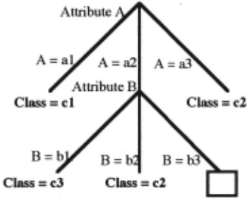
It is easy to see that node 1 corresponds to rule R 1 and that node 2-l corresponds to rule RJ. However, rule R2 does not appear itself in the tree; it cannot be generated. In fact node 2-2 corresponds to an over-specification of rule R2. Lastly, it appears that node 2-3 is empty, i.e. it does not cover any example of the learning set - and that node 3 is useless.
The reader will easily be convinced that, in this case, each of the possible decision trees generated with classic TDIS will contain empty, over-specific or useless nodes.
2.2- Production Rules Generation
Based on the lattice theory, the formal framework proposed here is able both to represent the activity of traditional TDIS and to eliminate their inherent limitations. For instance, it is possible to get rid of the bias described above.
The formalism is based on the use of two lattices, the so called relation lattice, noted ffi, which contains all the possible descriptions and the instance lattice, noted~. which corresponds to the set of parts of the training set. For instance, let us consider our training example: ((A = a2) & ( B = bl )) and ( D = dl) belong to ffi whereas {El E2 E4} and {E5, E7} belong to ~.
Afterwards, two correspondences between these two lattices are introduced, y: ffi ..... ~ and~: ~ ..... ffi.
y associates to each description the set of all the training examples which are covered by this description, so y(((A = a2) & (B = bl ))) = {E6, E7} and y((B = b2)) = {E4, E5} .
~ generates the most specific description common to all the examples of a subset of the training set. For instance, ~({El, F.3, E6}) = (B = bl) & (D = dl) and ~({EI. E2, F.3}) =((A= al) & (Class= cl)).
These two correspondences define what is called a Galois connection, whose properties enable an induction mechanism to be built. As an example, we can see that ~oy((A=al)) = ((A=al) & (Class=cl )). More generally, ~oy(d) gives the most specific description which is implied by the description d, i.e. the set of all the descriptors which are correlated with d in the learning set. This can then be simplified further, giving Affi((A=al )) = ~oy((A=al )) - (A=al) = (Class=cl ). The precise definition of Affi will be given in section 5 nevertheless, in a first approximation, the operator'-' can be assimilated to substraction. The reader can also verify that it is possible to have Affi (( B=b2 )) = (Class=c2) and f..m(((B=bl) & (A=a2))) = (Class=c3), which allows the generation of the knowledge base containing rules R 1, R2 and R3 since Affi(D) = d means If D Then d.
The following sections focus on the formalization of tllis induction technique. The CHARADE system [Ganascia 87] used the Boolean lattice formalism as a theoretical framework to generate production rule systems and was designed to express the learning strategies in a declarative way. We shall see here that it can be extended to any distributive lattice, .thus making it possible to take into account background knowledge by the use of distributive lattices properties. Since the proposed formalization encompasses all the previous algorithms, it is also possible to express many different learning strategies in declarative terms. In this way, the learning bias, i.e. the learning heuristics, can be considered as part of the knowledge and can be acquired in the same way as background knowledge.
3- Two Lattices
As announced above, the new formalization is based on the use of two lattices, the relation lattice and the instance lattice, which are described here.
3.1- Instance Lattice
The instance lattice ~ corresponds to the set of parts of the training set and is ordered by the inclusion relationship which is noted Si where A Si B means that A is included in B, i.e. B contains A, noted B ::>A.
Given two elements a and b, the least upper bound - noted (a Vi b) - and the greatest lower bound- noted (a Ai b) - correspond respectively to the classical union - i.e. u -and intersection -i.e. n - .
There is nothing to add to this description except that ~ is a Boolean lattice, i.e. a complemented distributive lattice.
3.2- Relation Lattice
The relation lattice ffl contains all the possible descriptions and is restricted here to an extended propositional logic using attribute-value items including linearly ordered and hierarchical attributes. It shall be seen in the following that all these attributes have useful properties for induction systems and their structure will be bound to the generalization space. But, let us not worry about the structure of these descriptions for the time being and concentrate on the ordering relation sg which corresponds to ~e generalization relationship where dt sg d2 means that d1 ts more general than rl2· Since a precise description of the structure of the relation space is not given here, no syntactic definition of the generalization relationship has been proposed. Let us just consider that it structures the relation space with a partial ordering and that any two elements of ffl have a greatest lower bound and a least upper bound. In other words, ffl is a lattice and, to be more precise, the greatest lower bound of two descriptions g1 and g2. i.e., (g1 1\g ~). corresponds to the generalization of those descriptions.
Without going into details, it is important to observe that the proposed framework is restricted to description language where there exists a unique least general generalization for each set of description. Therefore, this framework is adequate to represent classical TDIS [Quillian 1983] or Mitchell's version spaces [Mitchell 1982] but it is too restricted to formalize first order logic languages as they are used in inductive machine learning, for instance in [Muggleton and Feng 1990].
Let us note that (gl v g g2) is the most general description d such that gt sg d and g2 sg d. Therefore, it is easy to prove that, in the case of conjunctions of atomic propositions - noted 1\1 _, (g1 v g ~) is the logical conjunction of g1 and g2. i.e. (g1 vg g2) = (g1 AI g2). On the other hand, it is obvious that 1\g does not correspond to the logical conjunction.
4- Instance and Logical Closures
Once lattices ~ and ffl have been defined it is possible to define two closure operators on the poset ffl . The first one is related to correlations detected on the training set and is called the instance closure. The second is related to a set Q of logical implications and is the logical closure. The two closure operations are described here, the following section being concerned with how they can be used to induce production rules.
4.1- Instance closure
Let us begin by building two correspondences between the lattices~ and ffl .
The correspondence y: ffl - ~ associates to each description d of ffl the set of all instances of the training set which are covered by d. Since (gl 1\g g2) corresponds to the least general generalization of g1 and~. it is obvious that y(g 1 1\ g g2) = y(g I) u y(g2) = y(g I) vi y(g2)
~ : ~- ffl is the least general generalization. In other word, it is equivalent to making a set E of training instances corresponding to the least general generalization of the description of all the elements of E. This means that
Theorem: The correspondences y and ~ define a Galois connection between ffl and~.
Proof: It is only necessary to show that E Si y(d) if and only if d s:g ~). which follows from the definitions.
The correspondence d- ~(y(d)) is a closure operator since y and ~ define a Galois connection between ~ and ffl (see appendix for definition).
Notation: in the following, we shall note y(d) = d' and ~E)=E*
Theorem: ((d Ag dl)')* = (d')* Ag (d1')*
Proof: Here are the main steps of the proof, which follows directly from the three lemmas below:
Lemma 1: (dtAg d2) sg d if and only if d1 sg d and d2 s:g d. This lemma results from the distributivity of ffl .
Lemma 2: (dt Ag d2)' = dt' U d2'. 1t follows from the preceding lemma and from the definition of y.
Lemma 3: (E1 U E2)*= E1* U E2*· The proof uses the definition of~ and the properties of A g.
4.2- Logical closure
Let us now consider that ffl is a distributive lattice (see appendix for definition). It is now possible to build a closure operation relative to a set Q of logical implications corresponding both to background and to learned knowledge. Let us note that Q is given as a set of pairs of ffl which means that Q = {di ~ dj I ffl2 ::> (di. dj)}.
Definition: Let us define I(d, Q, n) as the set of deductions derived from d via Q after n inference steps.
Since we consider that ffl is a distributive lattice, it is known (see [Birkhoff 67] or [Gratzer 78]) that each element of ffl has a unique representation as a conjunction of 1\ irreducible elements of ffl . Let dl 1\ d2 1\ ... /\ dm be the representation of an element d of ffl :
Definition: The logical closure of d via Q, noted [d]Q, is the litnit of I(d, Q, n) when n- oo:
Theorem: The logical closure is a closure operator.
Proof. See [Ganascia 92].
Theorem: 'f(d 1· d2)Effl [d11\gd2]Q = [dtJQ Ag [d2]Q.
Proof: See [Ganascia 92].
5- INDUCTION
5.1- Introduction
As we have seen in the last section, there now exists two closure operations in 9l, the instance closure and the logical closure. The objective is to generate logical implications such that the logical closure and the instance closure are identical. In other words, logical implications must be induced and have to be introduced in Q, since these implications correspond to empirical regularities detected on the examples. As the logical closure is a closure operator, it is easy to prove that any addition to Q will increase every logical closure. In addition it would be desirable to eliminate redundancies, so some kind of simplification operator is needed. The easiest way is to introduce complementation into the lattice, which is equivalent to logical negation. However, there are two major drawbacks. The first one is related to the meaning of negation which is not clear at all in the case of induction. The second one is related to structural arguments: as we shall see in the following (see section 6), any complemented distributive lattice is atomic (Cf. [Birkhoff 67] or [Gratzer 78]) which prohibits the introduction of background knowledge directly in the lattice structure. To get over this it was necessary to introduce simplification using relatively complemented lattices or, more precisely the dual of a relatively complemented lattice which is interpreted as a Brouwerian logic, i.e. intuitionist logic (see [Birkhoff 67]). All these notions are described briefly in the next subsection, before going on to show how they are used to induce logical implications.
5.1- Brouwerian lattices
Definition: The pseudocomplement of a relative to b is the greatest element x such that a" x s: b. It is noted "a:b".
Since we need to simplify, to subtract, i .e. to build the difference between two descriptions, the dual of the relative pseudocomplement will defined and named "difference".
Definition : The difference "bla" is the dual of the pseudocomplement of a relative to b. In other words, it is the least x such that a v x ~ b . .
Definition: a Brouwerian lattice is a lattice where there exists a difference "bla" for each pair of elements (a, b). Theorem: Every Brouwerian lattice is distributive.
Proof: See [Birkhoff 67].
Theorem: Every finite distributive lattice is a Brouwerian lattice.
Proof: See [Birkhoff 67].
5.3- Implication generation
Once the difference has been defined, it is possible to build the smallest element which has to be added to the logical closure of a description d. It is the difference between the instance and the logical closure of d, i .e. (d')* I [d]Q and shall be named Affl(d, Q).
Therefore, it is obvious that adding d ~ Affl(d, Q) to Q makes Affl(d, Q U {d ~ Affl(d, Q)}) = 0. This means that it is possible to complete Q in order to make the logical closure equal to or greater than the instance closure.
For instance, in the case of the example given in section 2.1,Affi((A=al), 0) = ((A=al)')* I (A=al) =(Class=cl), we can generate the implication (A=al) ~ (Class=cl ). In the same way /..m((B=b2),0) =(Class=c2) which gives (B = b2) ~(Class = c2).
Now, let us imagine that the description ((A=a2) & ( B=b2)) is investigated. If ( B=b2) has already been explored then the implication (B=b2) ~ (Class=c2) will have been generated and inserted in Q, thus giving: A.m(((A = a2) & (B = b2)), {(B=b2)~ (Class=c2)}) = 0 whereas Affl(((A = a2) & (B = b2)), 0) =(Class=c2).
This way of generating implications is very general in the sense that it can generate all the possible implications corresponding to all the correlations observed on the training set. Most of the time, however, in machine learning, implications are restricted to a particular kind. For instance, in most TDIS algorithms, only implications which conclude on disjunctive classes Cj are generated, which is very easy to do with the new formalism by considering the least general generalization of Affl(d, Q) and all the classes Cj, i.e., Affi(d, Q) "g (( Class=c 1) "tf Class=c2) "g ... "g ( Class=c11)).
Going back to the example, let us envisage Affl((A=a3), 0) = ((B=b2) & (D=dl) & (Class=c2)). It contains two useless propositions ( B=b2) and ( D=dl ). If we build the least general generalization of 1-ffi((A=a3), 0) and ((Ciass=cl) "g (C/ass=c2) "g (Class=c3)) we get Affl (( A=a3 ), 0) "g (Class=cl) "g(Clas=c2) "g(Class=c3) = ((B=b2) v g(D=dl) v g (Class=c2))Ag (Ciass=cl) "s (Class=c2) "g (Class=c3) =(Class= c2).
In the following, this restriction will be ignored since the goal is just to have general limitation theorems to make the method efficient. However, the restriction must be kept in mind to get a clear idea of the power of the proposed framework.
Remark: As explained in 3.2, Vg and "g are relative to the generalization ordering S:g. There must not be any confusion; v g and "g have to be distinguished from logical conjunction and disjunction, "I (or&) and Vt. For instance, in the case of conjunction of atomic propositions, (gl vg g2) = (gl"l g'2) = (gl & g2) (see section 3.2).
5.4- Two Fundamental Theorems
This subsection proposes two fundamental theorems. The first one allows cuts in the description space once has been explored using a top-down strategy, i.e. from the general to the specific. The second offers the possibility to structure the relation space 9l using some background knowledge.
Theorem: If ((d 1 vg d2)')* = (dt')* then \fd ~g d1 Affl(d, Q) = 0 implies Affl(d vg d2. Q) = 0 .
Proof: d-(d')* being a closure operator, (((d1 ')* v g (d2')*)')* = ((dt vg d2)')* (see appendix for more details). Therefore (((d1')* vg (d2')*)')* = (dt')* follows directly from ((d1 vg d2)')* = (dt')*. More generally, when d ~g dt we have((dvgd2)')*=((dvgd1 vg<i2)')*=(((d')* vg((dt vg d2)')*)')*= (((d')* vg (dt')*)')* = (d')*. By defmition ofAffi(d, Q), if Affl (d. Q) = 0 then [d]Q ~ (d')*. Therefore [d v g d2]Q ~ [d) Q ~ (d')* = ((d v g d2)')* and then Affl(d Vg d2. Q) = 0 .
This theorem establishes that once <12 is covered· by d 1· i.e. once all the examples described by <12 are also described by d 1· descriptions like d v g d2, i.e. descriptions that are more specific than d1"1 d2 = d1 & d2 (see section 3.2) are useless. This is useful in cases of top-down learning strategies since it allows drastic cuts in the search. For instance, in the example (see section 2.1), it states that no description more specific than ((B = b3) & (A= al)) or((B = b3) & (D = d2)) has to be studied. Since the training set is too small it is not very convincing, but in the general case it is of crucial importance.
Theorem: 'v'(d, dt) Affi(d, Q) = 0 and Affi(d1, Q) = 0 imply f...!Jt(d Ag d1, Q) =0.
Proof: It follows from the definition of f...!Jt and form theorems given in the section 4.1 and 4.2. For more details see [Ganascia 1992]
This theorem allows the descriptions d Ag d 1 ... Ag dn to be cut out from the search space. The generation of logical implications makes A!Jt(d, Q) = A!Jt(d1,Q) = 0 for all disjonctions danddl, so Affl(d Ag d1. Q) =0 follows from the last theorem which then restricts the search space to A irreducible elements of the distributive lattice ffl . This restriction of the search space is crucial as we shall see in the next section.
6- Structure of Lattices
So far we have seen how to generate implications from a description d of !R. Taking the above theorems into account we shall now study the top-down exploration of m and then its structure. Remember that ffi is a distributive lattice. Using classical results from lattice theory it is possible to define a particular class of distributive lattices for which the complexity of the exploration is linear with the number of points, i.e. with the number of symbols belonging to m. These lattices, as we shall see, will play a central role in the structure of m. This section introduces this class of lattices
and goes on to show how it is possible to structure m.
Definition: A subset A of a poset X is said A-closed if and only if \fa=A., \fx x s: a==:. xEA.
Theorem: the free distributive lattice generated with n symbols, 0 and I, is dually isomorphic to the ring of all A closed subsets of {1, 2, ... , n}.
Proof: See [Birkhoff 67].
Definition: A poset X is said to be hierarchical if and only if \f (a, b) E x2 a~ b or as: b or {x/ x ~a and x ~ b} = {}. It means that a v b =if a~ b then a else if a s: b then b else I.
Theorem: Any element belonging to a distributive lattice L built on a hierarchical poset X is a conjunction of elements of the poset X.
Proof: See [Ganascia 92].
Therefore, in the case of distributive lattices built on hierarchical posets, only the conjunctions of elements of the hierarchical posets have to be considered. Moreover, in the last section it was proved that f...!Jt(d, Q) = 0 and Affi(d1. Q) = 0 imply f...!Jt(d Ag dt. Q) = 0. This means that, in the case of hierarchical posets, the only useful elements are the elements of the posets. In other words, using hierarchical posets the search space, i.e. the portion of the distributive lattice m which has to be explored, is linear with the number of elements of the poset X on which ffi is built. In practice, hierarchical posets correspond to attributes whose values are disjointed, linearly ordered or, more generally, partially ordered through a hierarchy.
Hierarchical posets correspond to hierarchies of propositions. It is not a sufficient representation since it was not possible to be restricted to just one attribute at a time. To increase the representational power, therefore, the product of distributive lattices built on hierarchical posets was introduced. Since it has been proved that the product of distributive lattices is a distributive lattice, the resulting relation lattice m is just the product of n hierarchical posets.
This structure could be interpreted in terms of machine learning as a set of attributes, each of which is a hierarchical attribute, i.e an attribute whose values belong to a hierarchy. This is exactly the structure of the representation that is used in [Mitchell 82] to represent the description space. It can also be seen as an extension of the attribute-value vectors as they are used in the classical TDIS algorithms like ID3, CN2, etc. One of the main advantages of this structure is that it allows a direct introduction of knowledge through hierarchies, whether this knowledge be composed of exclusive values, ordered attributes or general hierarchies.
In conclusion to this section concerning to the structure of the representation space, it is important to insist on two points related to the attribute-value representation which is commonly used in most cases of TDIS.
The first point is that classical TDIS can be extended to hierarchical and linearly ordered attributes, which allows the introduction of background knowledge. In relation to this first point, it should be noted that, due to the fact that the conclusions of implications do not have a special status, it is possible to organize classes in hierarchies, which allows some treatment of noise or approximation. However, this last point is beyond the scope of this paper.
The second point is that this formalism provides a strong mathematical framework justifying the representation used in TDIS. Again, the aim here is not to discuss questions of representation. After all , it is obvious that for many learning problems, attribute-value vectors - even with hierarchical attributes - do not constitute an adequate representation. Nevertheless, it is important to note that the proposed algebraic formalization of TDIS generalizes and justifies the classical representations which are commonly used both in classical TDIS and in other research such as [Mitchell 1982].
7- Conclusion and Future Work
The aim of this paper was to give a clear, intuitive presentation of the proposed formal framework which extends present TDIS with respect to learning strategies and representation. However it is not only of theoretical interest, and the next step is to use it in a practical manner along five lines .
The first point is to use it to test different learning strategies. It will be implemented so as to enable an easy introduction of many different learning strategies, thus allowing classical "ID-like" or "CN-like" strategies to be evaluated and compared with new ones.
It is possible to get multiple classification of the training set instances with this framework. This is related to the notion of redundancy which seems to be beneficial [Gams 89]. The second point is to give a systematic evaluation of tl1e usefulness of redundancy.
The third point concerns the ability to modify the learning bias and to express it as part of knowledge. A clear description of all the inputs of machine learning algorithms is required for their integration in a knowledge acquisition process. More precisely, a status has to be provided for each of tl1ese inputs. Expressed in terms of knowledge acquisition they can be acquired as part of the knowledge [Ganascia et Al. I992], which seems to be a promising approach, but it will have to be evaluated.
Much work has been done on noise in the case of TDIS. lbis has to be integrated in the new formalism, but it does not seem too difficult since pre-pruning is similar to cutting out nodes in the search space. New extensions to the model can also be investigated, for instance the use of hierarchical attributes. Some work has been done in this direction but it remains to be evaluated and will be the subject of the fourth point.
The fifth and final point is mainly of theoretical interest and involves examining the exact role of Brouwerian logic on which the new model is based. The introduction of Brouwerian logic was in fact a surprising spin-off considering that the only objective was to get a non atomic lattice as a description space. This question is directly related to the fact that distributive complemented lattices are necessarily atomic which means that the introduction of classical negation leads to a Boolean representation. Since the aim was to justify attribute-value representation a simplification operation has to be introduced without using complementation; the choice was pseudo-complementation. It now seems interesting to investigate the links between induction and intuitionism in more depth.
Appendix
lbis is an introduction to some basic notions of lattice theory. More details can be found in [Gratzer 78] and [Birkhoff 67]. ·
Definition: A poset is a partially ordered set, i .e. a set with a partial ordering relation :s:.
Definition: ro is a closure operation on the poset E if and only if:
- VXEE X :s: ro(X)
- VXEE ro(X) = ro(ro(X))
- V(X, Y)EE2 if X :s: Y then ro(X) :s: ro(Y)
Definition: An element X of E is closed for the closure operation ro if and only if ro(X)=X.
Definition: A lattice is a poset E such that there exists a least upper bound and a greatest lower bound for each pair (a, b) of elements of E. The least upper bound is noted (a v b) and the greatest lower bound (a 11 b).
- Theorem: ro being a closure operator on the lattice T, V(a, ~)Ef2 ro(ro(a) v ro(~)) = ro(a v ~).
- Definition: Let P and Q be two posets. Let X- X* and Y- Y' be two correspondences defined respectively on P and Q by ~: P- Q and y: Q - P and such that:
- I- V(x, xi) E P x :s: xi implies x* :l: xi*
- 2- V(y, yi) E Q y s yi implies y' :l: yi'
- 3- Vx E P x :s: (x*)' and Vy E Q y :s: (y')*
- X - X* and Y - Y' define a Galois connection between P and Q.
- Lemma: X- X* and Y - Y' define a Galois connection between P and Q, so VxEP ((x*)')* = x* and VyEQ ((y')*)' = y'.
Theorem: The following two applications x- (x*)' and y - (y')* are two closure operations.
- Definition: A lattice is distributive if and only if it satisfies (I) or (2):
- (I) V(x, y, z) x 11 (y v z) = (x 11 y) v (x 11 z)
- V(x, y, z) x v (y" z) = (x v y)" (x v z)
@inproceedings{ijcai1993p139,
  title     = {TDIS : an Algebraic Formalization},
  author    = {Ganascia, Jean-Gabriel},
  booktitle = {Proceedings of the Thirteenth International Joint Conference on
               Artificial Intelligence, {IJCAI-93}},
  publisher = {International Joint Conferences on Artificial Intelligence},
  editor    = {Ruzena Bajcsy},
  pages     = {1008--1014},
  year      = {1993},
  note      = {Machine Learning},
  url       = {https://ijcai.org/proceedings/1993/139},
}
TY - CPAPER TI - TDIS : an Algebraic Formalization AU - Ganascia, Jean-Gabriel T2 - Proceedings of the Thirteenth International Joint Conference on Artificial Intelligence, IJCAI-93 PB - International Joint Conferences on Artificial Intelligence PY - 1993 SP - 1008 EP - 1014 UR - https://ijcai.org/proceedings/1993/139 ER -Copied
Machine-readable versions of this paper, for tools and AI agents:
 Welcome
 Future Conferences
 AI Journal Division
 IJCAI Proceedings
 About IJCAI
 IJCAI Awards