
Induction of Oblique Decision Trees
Proceedings of the Thirteenth International Joint Conference on Artificial Intelligence. Machine Learning. Pages 1002-1006.
© 1993 International Joint Conferences on Artificial Intelligence
Abstract
This paper introduces a randomized technique for partitioning examples using oblique hyperplanes. Standard decision tree techniques, such as ID3 and its descendants, partition a set of points with axis-parallel hyperplanes. Our method, by contrast, attempts to find hyperplanes at any orientation. The purpose of this more general technique is to find smaller but equally accurate decision trees than those created by other methods. We have tested our algorithm on both real and simulated data, and found that in some cases it produces surprisingly small trees without losing predictive accuracy. Small trees allow us, in turn, to obtain simple qualitative descriptions of each problem domain.
- [Baum and Haussler, 1989] E. Baum and D. Haussler. What size net gives valid generalization? Neural Com- putation, 1:141-160, 1989.
- [Blum and Rivest , 1988] A. Blum and R. L. Rivest . Training a 3-node neural network is np-complete. In Proceedings of the First ADM Workshop on the Com- putational Learning Theory, pages 9-18, Cambridge, MA, 1988.
- [Breiman et al., 1984] L. Breiman, J . Friedman, R. 01- shen, and C. Stone. Classification and Regression Trees. 1984.
- [Duda and Hart, 1973] R. Duda and P. Hart. Pattern Classification and Scene Analysis. Wiley, 1973.
- [Heath, 1992] D. Heath. A geometric framework forma- chine learning. PhD thesis, The Johns Hopkins Uni- versity, Baltimore, MD, 1992.
- [Hyafile and Rivest, 1976] L. Hyafile and R. Rivest. Constructing optimal binary decision trees is np- complete. Information Processing Letters, 5(1):15-17, 1976.
- [Judd, 1988] J . S. Judd. On the complexity of load- ing shallow neural networks. Journal of Complexity, 4:177-192, 1988.
- [Lin and Vitter, 1991] J . H. Lin and J . S. Vitter. Com- plexity results on learning by neural nets. Machine Learning, 6:211-230, 1991.
- [Mangasarian et al., 1990] Mangasarian, R. Setiono, and W. Wolberg. Pattern recognition via linear pro- gramming: Theory and application to medical diag- nosis. SIAM Workshop on Optimization, 1990.
- [Mingers, 1989] J. Mingers. An empirical comparison of pruning methods for decision tree induction. Machine Learning, 4:227-243, 1989.
- [Odewahn et al., 1992] S. C. Odewahn, E. B. Stockwell, R. L. Pennington, R . M. Humphreys, and W. A. Zu- mach . Automated star/galaxy discrimination with neural networks. Astronomical Journal, 103(1):318- 331, 1992.
- Quinlan, ] J .R. Quinlan . Simplifying decisoin trees. In- ternational Journal of Man-Machine Studies, 27:221- 234 .
- [Quinlan, 1986] J .R. Quinlan. Induction of decision trees. Machine Learning, 1(1):81-106, 1986.
- [Salzberg, 1991] S. Salzberg. Distance metrics for instance-based learning. In Methodologies for Intel- ligent Systems: 6th International Symposium, ISMIS '91, pages 399-408, New York, 1991. Springer-Verlag.
- Utgoff and Brodley,] P. Utgoff and C. Brodley. An in- cremental method for find multivariate splits for deci- sion trees. In Proceedings of the Seventh International Conference on M athine Learning, pages 56-65, Los Altos, CA . Morgan Kaufmann.
- [Utgoff, 1989] P. Utgoff. Incremental induction of deci- sion trees. Machine Learning, 4(2):161-186, 1989.
- [Wiess and Kapouleas, 1989] S. Wiess and I. Kapouleas. An empirical comparison of pattern recognition, neu- ral nets, and machine learning classification methods. In Proceedings of the Eleventh IJCAI, Detroit, MI, 1989. IJCAI
- Morgan Kaufmann.
References were extracted automatically from the PDF and may contain errors.
Full text extracted automatically from the PDF; figures, tables and equations may differ. The PDF is the version of record.
1 Introduction
Decision trees have been used successfully for many dif ferent decision making and classification tasks. A num ber of standard techniques have been developed in the machine learning community, most notably Quinlan's ID3 (1986) and Breiman et a/. 's CART (1984) . Since the introduction of these algorithms, numerous variations and improvements have been put forward, including new pruning strategies (e.g., Quinlan, 1987) and incremental versions of the algorithms (Utgoff, 1989). Many of these refinements have been designed to produce better de cision trees; i.e., trees that were either more accurate classifiers, or smaller trees, or both.
The main goal of our research to produce decision trees that provide small, accurate models for a set of data. Many applications, including the ones discussed in this paper, could substantially benefit from reducing the size of the tree. In particular, a small tree will provide ex perts with important qualitative descriptions that may be used in real-world applications. ·
Most decision tree algorithms use axis-parallel hyper planes to partition a dataset. That is, if each example is characterized as a vector of numbers (z1, z2 , ... , Zd), the internal nodes of the tree will contain tests of the form z; > k. The task of the decision tree algorithm is to choose good values for i and k at each node. These tests are equivalent to axis-parallel hyperplanes. In order to provide the best fit to a dataset, we have chosen a more general representation: our algorithm uses oblique (non axis-parallel) hyperplanes to partition the examples. In other words, each node of the tree contains a hyperplane that can take any orientation in feature space. Because finding these hyperplanes turns out to be computation ally expensive, we introduce a randomized technique for selecting good hyperplanes. The goal of our work is to find smaller decision trees that provide a better fit to the data, and therefore are likely to be more accurate. Our results show that our method finds strikingly small trees for some datasets.
In the sections that follow, we present the following results:
- A new randomized approach for computing decision trees using non-axis-parallel hyperplanes. This use of randomized algorithms is new in the context of decision tree induction.
- A new NP-completeness result for the complexity of finding oblique hyperplanes. This result also pro vides a complexity bound for many other learning methods.
- Experiments demonstrating that our algorithm can produce very small oblique decision trees with ac curacies comparable to those of large axis-parallel trees.
Our new algorithm, which is based on simulated anneal ing, produces a different decision tree each time it is run on a given dataset. This property, a direct consequence of randomization, is a major advantage in light of the fact that finding the best tree is NP-complete. In order to find a good tree, we train the algorithm repeatedly on a fixed set of data, and retain only the smallest tree. As we will show in Section 5, the program frequently finds very small and accurate trees. Our experiments compare our program, which we call SADT 1 , to other decision tree algorithms (including ID3) on both simu lated and real data.
2 Complexity of finding good trees
Standard decision tree algorithms work recursively; i.e., given a set of examples, they generate a test which splits the examples into two subsets. They then recurse on the subsets, continuing to generate tests until some stopping criterion is satisfied.
1 Simulated Annealing of Decision Trees
The main difference between our problem and the gen eration of axis-parallel trees is that our tests can take the more general form of an oblique hyperplane. Stan dard decision tree algorithms use exhaustive search to find the "best" hyperplane (the criteria used to define the best test is described below). Because there are only a small number of distinct axis-parallel hyperplanes (i.e., for n examples and d attributes, there are d( n- 1) place ments), this can be done quite efficiently. However, the number of distinct partitionings of the same set of exam ples that can be induced with a single oblique hyperplane is O(nd), so that the straightforward approach of consid ering all possible tests is too expensive for many reason able values of n and d. For example, one of the datasets used in Section 5 has n = 4164 and d = 14. This obser vation led us to consider the computational complexity of finding the best test when tests are represented by oblique hyperplanes. We found that for reasonable def initions of "best," this problem is NP-complete; i.e., it probably has no polynomial time algorithm. This result implies that exhaustive search is not feasible for many datasets.
Theorem 2.1: Let the energy e of a l1yperplaiJe be de fined by the sum-minority energy measure (defiiJed be low). Given two point sets K1 and K2 aiJd a value k, the problem of determining if tl1ere is a hyperplaiJe sucl1 that e $ k is NP-complete.
For a proof of this theorem, see [Heath, 1992]. Note that this theorem says that finding even one optimal hyperplane is hard; clearly, then, building a whole tree is even harder.
It is worth noting that there do exist energy measures for which finding the best hyperplane is possible in poly nomial time. See [Duda and Hart, 1973] for a description of different techniques of generating hyperplanes in the absence of linear separability.
2.1 Finding approximate solutions
It is clear that by abandoning the restriction to axis parallel hyperplanes, we have made the problem of build ing decision trees considerably harder. Even at one par ticular node of the decision tree, we can not be sure of finding the best split, even if we define the goodness of the split in a simple, local way. What saves us from dis aster is that the best tree may not use the best first split anyway! This suggests that a randomized method, one that tries a range of good (but not best) initial splits and produces a set · of alternative trees, might produce good approximate solutions. This is exactly the approach we have taken.
As with many NP-hard optimization problems, our best strategy is to look for approximations or good heuristic solutions. There are several standard ap proaches for computationally hard optimization prob lems. Such possibilities include local search or gradient descent on the cost function. Typically, such methods suffer from the problem of getting stuck in local max ima. Two standard solutions to this problem are applying multiple local searches and applying a stochastic optimization approach such as simulated annealing. Per ceptron trees, introduced in Utgoff and Brodley (1990) can be seen as an instance of applying multiple local searches to the problem of finding a good first split. Once one good split is found, they recursively apply the pro cedure (i.e., multiple local-search) to the resulting par titions of the data. Breiman et al. (1984) use a single application of a local improvement algorithm. They it erate on dimensions, finding the best perturbation in the dimension until no improvement can be made. Both al gorithms are deterministic and output a single tree. Our algorithm produces a stream of different trees for a given training set. We can generate any number of these trees during training, and choose, for example, the smallest one for experimentation on the test-set.
It is well-understood that finding the best first split will not necessarily produce the smallest decision tree (i.e., the smallest tree may have a non-optimal root node) . Allowing randomization in the procedure that finds the best first split, and producing many alterna tive trees, increases the probability of finding good trees. We believe that randomization is an important technique in the context of inductive learning procedures. Since none of the known deterministic learning procedures are guaranteed to generate good minimum-size representa tions (trees), the introduction of randomization gives us a higher probability of finding such representations.
Thus one of the principal claims we wished to in vestigate experimentally was whether, when an optimal tree cannot be found, randomized algorithms may pro duce better decision trees than simple deterministic al gorithms. Given that any algorithm to find oblique deci sion trees cannot be guaranteed to find the best tree and still run in reasonable time, we decided that we needed an algorithm that could produce many different trees. Our SADT algorithm produces a different tree each time it runs. We sometimes run it hundreds of times on a given dataset, choosing the minimum size tree as the best one. Our argument is that picking the best of many solutions produced by a randomized algorithm may be preferable to using an algorithm, even a very clever one, that only produces one solution.
3 The simulated annealing algorithm
The basic outline of our algorithm is the same as that of most other decision tree algorithms. That is, we find a hyperplane to partition the training set and recurse on the two partitions. Here we describe the search for a good hyperplane.
In our implementation, d-dimensional hyperplanes are stored in the form H(x) = hd+l + :L:t=l hiXi, where H = {h1, h2, ... , hd+d is the hyperplane, x = (x1, x2, ... , xd) is a point, and hd+l represents the constant term. For example, in the plane the hyperplane is a line and is represented in the familiar ax + by + c = 0 form. Clas sification is done recursively. To classify an example, compare it to the current hyperplane (initially this is the root node). If an example pis at a non-leaf node la beled H(x), then we follow the the left child if H(p) ~ 0; otherwise we descend to the right child.
The first step in our algorithm is to generate an ini tial hyperplane. The initial hyperplane we generate is always the same and is not tailored to the training set. We simply wanted to choose some hyperplane that was not parallel to any of the axes, so we used the hyper plane passing through the points where x; = 1 and all other Xj = 0, for each dimension i. In particular, the initial hyperplane may be written in the above form as h; = 1 for 1 ~ i ~ d and hd+l = -1 since H(x) = 0 for each of these points. Thus in 3-D, we choose the hyperplane which passes through (1, 0, 0), (0, 1, 0), and (0, 0, 1). Many other choices for the initial hyperplane would be equally good. Once the annealing begins, the hyperplane is immediately moved to a new position, so the location of the initial split is not important.
Next, the hyperplane is repeatedly perturbed. If we denote the current hyperplane by H {h1, h2, ... , hd+d, then the algorithm picks one of the h; 's randomly and adds to it a uniformly chosen random variable in the range [-0.5, 0.5). Using our goodness measure (described below), we compute the energy of the new hyperplane and the change in energy ~E.
If ~E is negative, then the energy has decreased and the new hyperplane becomes the current split. Other wise, the energy has increased (or stayed the same) and th~ ~ew hype~lane bec~mes the current split with prob ablhty e-t:.Ef where T 1s the temperature of the system. The system starts out with a high temperature that is reduced slightly with each move. Note that when the change in energy is small relative to the temperature, the probability of accepting the new hyperplane is close to 1, but that as the temperature becomes small, the probability of moving to a worse state approaches 0.
In order to decide when to stop perturbing the split, we keep track of the split that generated the lowest en ergy seen so far at the current node. If this minimum energy does not change for a large number of iterations (we used numbers between 3000 and 30000 iterations in our experiments), then we stop making perturbations and use the split that generated the lowest energy. The recursive splitting continues until each node is pure; i.e., each leaf node contains only points of one category.
3.1 Goodness criteria
Our SADT algorithm can work with any goodness crite rion, and we have experimented with several criteria. For detailed discussions of these measures, see Heath [1992]. In these earlier studies, the sum-minority goodness mea sure generated smaller, more accurate trees than the oth ers we tested. As a result, we chose the sum-minority goodness measure for the experiments described here. This measure is defined as follows.
Consider a set of examples X, belonging to 2 classes, u and v. A hyperplane divides the set into two subsets X1 and X2. For each subset, we find the class that ap pears least often. We say that these are the minority categories. If x. has few examples in its minority cate gory C1, then it is relatively pure. We prefer splits that are pure; i.e., splits that generate small minorities. Let the number of examples in class U (class v) in X1 be U1 ( v1) and the number of examples in class u (class v) in x2 be U2 ( v2)· To force SADT to generate a relatively pure split, we define the sum-minority error measure to be min(u1,v1) + min(u2,v2). For a description of this and other error measures, see [Heath, 1992].
3.2 Taking advantage of randomization
We believe randomization in learning algorithms can eas ily be used to advantage. Because SADT constructs dif ferent trees every time, it is possible to run it multiple times and pick a tree or set of trees that has some ad vantage over a more "average" tree. For example, to minimize tree size, one can run SADT several times and choose the smallest tree it creates.
Another way we can benefit from randomization is to take a set of SADT trees, and combine their classifica tions by taking the plurality. In hi-classification prob lems, this reduces to taking the majority. For example, if we have 5 trees, and 3 classify an example as "0," and the other two classify it as "1," then we predict the example belongs to class "0."
The premise behind this idea is that any one tree may not capture the target concept completely accurately, but will approximate it with some error. This error dif fers from tree to tree. By using several trees and taking the plurality, we hope to overcome this type of error.
4 An example in the plane
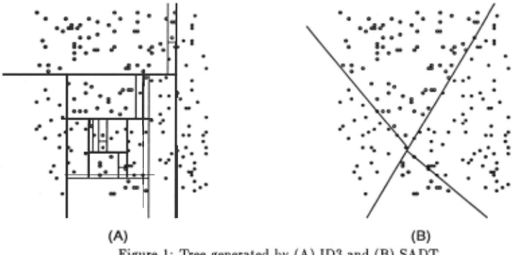
To illustrate the possible advantages that SADT offers, we demonstrate its use on an artificial dataset containing 200 examples in two classes, chosen uniformly from a two-dimensional space. We labeled the points according to a partitioning with three non-axis-parallel lines. Thus, the optimal partitioning (and the optimal tree) required three oblique "splits."
Figure 1 shows the tree generated by ID3 and one of the trees generated by SADT. The tree generated by ID3 did not fit the data very well, because the correct parti tions were oblique lines. We ran one hundred trials with each of our goodness measures, and kept the smallest tree as the best . This example shows that, at least for simple problems, SADT can perform very well.
5 Experiments
5.1 Applying SADT to cancer diagnosis
For our first experiment, we ran SADT on a real dataset that has been the subject of other machine learning stud ies; in particular, it was the subject of experiments that partitioned the data using oblique hyperplanes (Man gasarian et al., 1990). This dataset contains 470 exam ples of patients with breast cancer, and the diagnostic task is to determine whether the cancer is benign or ma lignant. Each example has 9 numeric attributes, hence our decision trees used hyperplanes in 9-D.
Mangasarian's method uses linear programming to find pairs of hyperplanes that partition the data. The al gorithm finds one pair of parallel hyperplanes at a time, and each pair can be oriented at any angle with respect to all other pairs. The resulting model is a set of oblique hyperplanes, similar though not identical to an oblique decision tree.
. .. , . 0
| Algorithm | Accuracy on Test Data (%) | Number of Hyperplanes |
|---|---|---|
| SADT | 97 | 1 |
| 103 | 83 | 30 |
| Mangasarian et al. | 97 | 16 |
| EACH | 95 | |
| Nearest Neighbor | 94 |
Because Mangasarian et al. received the data as they were collected in a clinical setting, their experimental design was very simple. They trained their algorithm on the initial set of 369 examples. Of the 369 patients, 201 (54.5%) had no malignancy and the remainder had confirmed malignancies. On the next 70 patients to en ter the clinic, they used their algorithm for diagnosis, and found that it correctly diagnosed 68 patients. We used 68/70 = 0.97 as a rough estimate of the accuracy of Mangasarian et al. 's method. They then re-trained their algorithm using the 70 new patients, and reported that it correctly cl~sified all of the next 31 patients to enter the clinic. Mangasarian reported that his program's out put was being used in an actual clinical setting. Using the same dataset with a more uniform experimental de sign, Salzberg reported that the EACH hyper-rectangle program produced 95% classification accuracy, and ! nearest-neighbor had 94% accuracy (Salzberg, 1991) .
We imitated Mangasarian et al. 's experiment by using the same 369 examples from their initial trial to produce decision trees, which we then tested on the final 101 patients. It is not possible to show a nine-dimensional partitioning here, but our results and some comparisons are summarized in Table 1.
Mangasarian's model used 8 pairs of hyperplanes - 16 hyperplanes - to model the data. With SADT we were able to determine that the same accuracy can be attained with a single hyperplane. Our method uses a significantly smaller number of oblique planes, and produces comparable accuracy. The axis-parallel hyper planes produced by ID3 made a much poorer classifier for this dataset - the tree was much larger and was less accurate than the SADT tree. As a side note, some of the larger trees generated by SADT scored 100% on the test set. The smallest such "perfect" tree contained 6 hyperplanes.
| Algorithm | Accuracy (%) | Std Dev | Tree Size | Std Dev |
|---|---|---|---|---|
| SADT | 94.9 | 3.47 | 4.58 | 2.0 |
| 103 | 88.1 | 9.89 | 27.8 | 4.7 |
In addition, we ran a ten-fold cross-validation trial on the same set of data. In an x-fold cross-validation trial, we divide the dataset into x approximately equal sized subsets and perform x experiments. For each set s, we train the learning system on the union of the remaining x - 1 sets and test on set s. The results are averaged over these x runs. The results of these tests are shown in Table 2. For each of the ten training- and test-set pairs, we performed thirty-six trials. That is, each value in Table 2 is the average of 360 values and should be more indicative of the true accuracy on the problem. The SADT trees are somewhat more accurate than the axis parallel trees. The size of the trees generated by SADT is considerably less that that of the trees generated by 103. We note that there are different ways in which the size of trees can be measured. In this paper, we equate tree size with the number of hyperplanes, regardless of the description complexity of the hyperplanes.
5.2 Identifying stars and galaxies
In order to study the performance of SADT on larger datasets, we ran several experiments using astronomical irnage data collected with the University of Minnesota Plate Scanner. This dataset contains several thousand astronomical objects, all of which are classified as either stars or galaxies. Odewahn et al. [1992] used this dataset to train perceptrons and backpropagation networks.
| Algorithm | Dataset | Accuracy (%) | Std Dev | Tree Size | Std Dev |
|---|---|---|---|---|---|
| SADT | Br1ght | 99.0 | 0.48 | 7.03 | 2.2 |
| ID3 | 99.0 | 0.63 | 37.7 | 2.7 | |
| SADT | D1m | 94.0 | 1.2 | 27.6 | 13 |
| ID3 | 94.7 | 1.1 | 260 | 150 |
Although we did not have access to the exact train ing and test set partitions used by Odewahn et al., we approximated the data using the same filtering of data from the same source. Although our results may not be completely comparable to theirs, we include them to show that both learning methods produce similar accu racies. Our results were generated by averaging nineteen 10-fold cross-validation trials.
We experimented on two different subsets of the astro nomical data. One set is comprised of dim objects, the other of bright objects. Bright objects tend to be easier to classify. The bright dataset consists of 4164 exam ples; there are 4652 examples in the dim dataset . Each example has fourteen real-valued attributes and a label of either "star" or "galaxy." Approximately 35% of the examples are galaxies.
Classification results are shown in Table 3. Odewahn et al. [1992] obtained accuracies of 99.7% using back propagation on the bright dataset and 92.2% on the dim dataset. We obtained a cross-validated accuracy of 99.1% with a perceptron on the bright dataset . Note that a perceptron can be considered a tree of size 1. This implies that SADT trees, despite their small size, could still benefit from pruning. The accuracy of the trees generated by SADT and those generated by ID3 was ap proximately the same in both cases. However, SADT was able to find much smaller trees than ID3.
5.3 Classifying irises
Fisher's [1936] iris data is a well known dataset, and many common learning techniques have been applied to it. The data consists of 150 examples, 50 each of three different types of irises: setosa, versacolor, and virginica. Each example is described by numeric measurements of width and length of the petals and sepals.
We performed thirty-five 10-fold cross-validation tri als using SADT. Averaged results are shown in Table 4, along with 10-fold cross-validation trials for ID3. Weiss and Kapouleas [1989] obtained accuracies of 96.7%, 96.0%, and 95.3% with backpropagation, nearest neigh bor, and CART, respectively, using leave-one-out trials, i.e., 150-fold cross validation.
Once again, we note that the accuracy of SADT is comparable to that of other learning techniques. The trees generated by SADT tend to be somewhat smaller and more accurate on average than those of ID3.
| Algorithm | Accuracy (%) | Std Dev | Tree Size | Std Dev |
|---|---|---|---|---|
| SADT | 94.7 | 5.99 | 4.24 | 1.5 |
| ID3 | 90.0 | 8.5 | 7.8 | 1.7 |
| Dataset | Technique | Glassijication Accuracy | Tree Size |
|---|---|---|---|
| Cancer malignancy | average smallest | 94.9 95.1 | 4.58 1.90 |
| Sta~/ galaxy Bright | average smallest | 99.0 99.1 | 7.03 3.80 |
| Star[galaxy Dim | average smallest | 94.0 94.2 | 27.6 15.2 |
| Iris | average smallest | 94.7 96.6 | 4.24 2.20 |
6 Pruning SADT trees
The problem of generating small decision trees through choice of a stopping criterion or energy measure has been considered difficult. See, for example, [Breiman, et al., 1984] . The approach commonly used for standard deci sion trees is to first generate a tree that correctly classi fies every training example, and use another procedure, pruning, to reduce the size of the tree. See [Mingers, 1989] for an overview of several decision tree pruning methods. The results we present in our paper are for unpruned trees. It turns out that some pruning methods work well on our oblique trees. A comparison of pruning strategies for SADT can be found in [Heath, 1992].
7 Predicting using smallest trees
One advantage of randomization is that SADT can gen erate many different trees to model a dataset, and then use some additional criterion to decide which tree to use for classification. We believe that smaller trees provide a qualitatively better description of a domain, and we therefore used tree size as a criterion for picking trees. Table 5 shows a comparison of predictive accuracy and tree size for all four of our datasets using two crite ria. Our default method, average, was to use SADT to generate approximately 200 different trees, and the results in the table give the average accuracy of all these trees. However, if we simply pick the smallest tree gen erated by the algorithm, performance improves slightly, as shown in the table. The benefit to this technique is that we can obtain smaller trees with no loss (and per haps even an increase) in accuracy. (Each line in the table represents a 10-fold cross-validation study; there fore, accuracy and tree size are averages over 10 runs.)
8 Summary of Results
We have developed an algorithm for generating oblique decision trees, in which decisions are linear threshold functions of example attributes. We have shown that for reasonable goodness measures, finding best splits is probably not possible in polynomial time.
This result differs from most previous NP-complete ness results addressing learning complexity. Hyafil and Rivest (1976) showed that finding a decision tree that minimizes expected classification time is NP-hard. Blum and Rivest (1988) show that learning is difficult even when trying to train a neural network with only 3 nodes. Several other published results have considered the complexity of exact learning, namely, finding a cir cuit, formula or neural network consistent with a dataset. (See, e.g., Baum and Haussler, 1989; Blum and Rivest, 1988; Judd, 1988; and Lin and Vitter, 1991.) All of these results require at least a two level circuit or neural net work, since the problem of learning with a single layer can be solved using linear programming. Unlike the pre vious results, which apply to exact learning, our result addresses approximate learning. We show that the ap proximate learning problem is NP-complete even for the simplest model of a neural mechanism: the perceptron.
This has forced us to examine methods of finding good (as opposed to best) splits. Our experiments have shown that simulated annealing works well as a method for gen erating oblique decision trees, in that it generates trees with fewer tests, while maintaining classification accu racy. We have compared our methods to others on both real and artificial data, in order to give a broad overview of how well the methods work. We plan to explore these techniques further by using different annealing methods and different goodness criteria. We are also develop ing randomized geometric algorithms that will be more efficient than annealing. In this paper, our goal was to test the thesis that smaller trees generate good decisions. This justifies the effort to seek efficient algorithms for finding good oblique decision surfaces in a decision tree.
If construction of a good classifier is more important than producing a concise representation, then one might use SADT to generate a set of trees, and then use the majority vote for classification. We have experimented with this and other ideas (Heath,-1992], but these results are not included in the interest of brevity.
To summarize, SADT was able, for the datasets we used in our experiments, to generate quite small trees. We consider this to be its main advantage over other decision tree algorithms.
Acknowledgements
The authors wish to thank David Aha for providing comments and relevant references. This research was supported in part by the Air Force Office of Scientific Research under Grant AFOSR-89-0151, and by the Na tional Science Foundation under Grant IRI-9116843.
@inproceedings{ijcai1993p138,
  title     = {Induction of Oblique Decision Trees},
  author    = {Heath, David G. and Kasif, Simon and Salzberg, Steven},
  booktitle = {Proceedings of the Thirteenth International Joint Conference on
               Artificial Intelligence, {IJCAI-93}},
  publisher = {International Joint Conferences on Artificial Intelligence},
  editor    = {Ruzena Bajcsy},
  pages     = {1002--1006},
  year      = {1993},
  note      = {Machine Learning},
  url       = {https://ijcai.org/proceedings/1993/138},
}
TY - CPAPER TI - Induction of Oblique Decision Trees AU - Heath, David G. AU - Kasif, Simon AU - Salzberg, Steven T2 - Proceedings of the Thirteenth International Joint Conference on Artificial Intelligence, IJCAI-93 PB - International Joint Conferences on Artificial Intelligence PY - 1993 SP - 1002 EP - 1006 UR - https://ijcai.org/proceedings/1993/138 ER -Copied
Machine-readable versions of this paper, for tools and AI agents:





