
Efficient Pruning Methods for Separate-and-Conquer Rule Learning Systems
Proceedings of the Thirteenth International Joint Conference on Artificial Intelligence. Machine Learning. Pages 988-993.
© 1993 International Joint Conferences on Artificial Intelligence
Abstract
Recent years have seen increased interest in systems that learn sets of rules. The goal of this paper is to study the degree to which "separate and conquer" rule learning induction methods scale up to large, real-world learning problems. In particular, we study the asymptotic complexity of rule induction on large training sets in the presence of noise. We present formal arguments and experimental data supporting the claim that existing methods do not scale up well on noisy data . We then present a solution in the form of new pruning techniques that dramatically improve the runtime of rule induction methods with no loss in accuracy: formal analysis shows an improvement in asymptotic time complexity, and experiments show an order-of-magnitude speedup on a set of benchmark problems while obtaining slightly more accurate hypotheses.
- [Ali and Pazzani, 1993] Kamal Ali and Machael Paz- zani. HYDRA: A noise-tolerant relational concept learning algorithm. In Proceedings of the 19th Inter- national Joint Conference on Artificial Intelligence, Chambery, France, 1993. IJCAI
- [Brunk and Pazzani, 1991] Clifford Brunk and Michael Pazzani. Noise-tolerant relational concept learning al- gorithms. In Proceedings of the Eighth International Workshop on Machine Learning, Ithaca, New York, 1991.
- Morgan Kaufmann. [Catlett, 1991] Jason Catlett. Megainduction: a test flight. In Proceedings of the Eighth International Workshop on Machine Learning, Ithaca, New York, 1991.
- Morgan Kaufmann. [Clark and Niblett, 1989]
- P. Clark and T. Niblett. The CN2 induction algorithm. Machine Learning, 3(1), 1989.
- [Cohen, 1991] William W. Cohen. Grammatically bi- ased learning: learning Horn theories using an explicit antecedent description language. AT&T Bell Labs Technical Memorandum . Available from the author on request, 1991.
- [Cohen, 1992a] William W. Cohen. Compiling knowl- edge into an explicit bias. In Proceedings of the Ninth 994 Machine Learning International Conference on Machine Learning, Ab- erdeen, Scotland, 1992.
- Morgan Kaufmann .
- [Cohen, 1992b] William W. Cohen . Efficient pruning methods for separate-and-conquer rule learning sys- tems. AT&T Bell Labs Technical Memorandum . Available from the author on request, 1992.
- [Pagallo and Hassler, 1990] Giulia Pagallo and David Hassler. Boolean feature discovery in empirical learn- ing. Machine Learning, 5(1), 1990.
- [Pazzani and Kibler, 1992] Michael Pazzani and Dennis Kibler. The utility of knowledge in inductive learning. Machine Learning, 9(1), 1992.
- [Quinlan, 1987] J . Ross Quinlan. Simplifying decision trees. International Journal of Man-Machine Studies, 27:221-234, 1987.
- [Quinlan, 1990] J. Ross Quinlan. Learning logical defi- nitions from relations. Machine Learning, 5(3), 1990.
- [Schaffer, 1992] Cullen Schaffer. Spare data and the ef- fect of overfitting avoidance in decision tree induction . In Proceedings of the Tenth National Conference on Artificial Intelligence, San Jose, California, 1992. MIT Press.
- [Weiss and Indurkhya, 1991] Sholom Weiss and Nitin Indurkhya. Reduced complexity rule induction . In Proceedings of the 12th International Joint Conference on Artificial Intelligence, Sydney, Australia, 1991. IJCAI
- Morgan Kaufmann. [Weiss and Kulkowski, 1990] Sholom Weiss and Casmir Kulkowski. Computer Systems that Learn. Morgan Kaufmann, 1990.
References were extracted automatically from the PDF and may contain errors.
Full text extracted automatically from the PDF; figures, tables and equations may differ. The PDF is the version of record.
1 Introduction
Of number of systems exist that learn sets of if-then rules. Many rule learning systems generate hypotheses using a greedy strategy in which rules are added to the rule set one by one in an effort to form a small cover of the positive examples; each rule, in turn, is created by adding one condition after another to the antecedent until the rule is consistent with the negative data. This greedy approach to building rule sets has been termed separate and conquer, by analogy with the divide and conquer approach commonly used in top-down decision tree induction [Pagallo and Hassler, 1990].
Recent years have seen increased interest in rule learn ing systems in general, and separate-and-conquer rule learning systems in particular. One reason is that the rule sets have a natural and familiar first order version, namely Prolog predicates; the separate-and conquer approach has been quite successful in learning various restricted sublanguages of Prolog [Cohen, 1992a; Quinlan, 1990; Pazzani and Kibler, 1992]. Rule sets are also representationally more powerful than competing representations such as decision trees; this is reflected in the fact that rule induction systems significantly outperform standard decision tree induction systems on many problems [Pagallo and Hassler, 1990; Quinlan, 1987; Weiss and lndurkhya, 1991]. Finally, many sorts of prior knowledge about a learning problem can be communi cated to a rule induction system by providing appro priate constraints on the form of induced rules [Cohen, 1991; Cohen, 1992a].
The goal of this paper is to study the degree to which rule set induction methods scale up to large, real-world learning problems. In . particular, we will study the asymptotic complexity of rule induction in the presence of two phenomena common in real-world datasets: large training set size and noise. In Sections 2 and 3, we show that existing methods do not scale up well, presenting evidence to this effect in the form of both experimental results and formal argument. In Section 4 we propose some solutions to these problems. These solutions are then evaluated in Section 5. We show that our prun ing methods dramatically improve the asymptotic time complexity of rule induction with no apparent loss in accuracy.
2 Rule induction: does it scale up?
2.1 Noise-free rule induction
In this paper, we will use as our experimental testbed pFOIL, which is a propositional version of the rule in duction system FOIL [Quinlan, 1990] . Briefly, pFOIL is a top-down, "separate-and-conquer" rule induction sys tem; it builds a rule set greedily by adding one rule after another to an initially empty rule set until all positive examples are covered. Each rule in turn is built using an other greedy strategy, starting with a maximally-general rule and repeatedly specializing it by adding a single condition until the rule covers no negative examples. The specialization process is based on information-gain heuristics. 1
On multi-class problems, pFOIL learns a set of rules for each class that separates the examples of that class from examples of all other classes. When classifying, conflicts between rules are currently resolved by choosing the classification suggested by the rule which is most ac curate on the training data. This strategy is also followed on two-class problems: for example, on the mushroom problem described below, pFOIL learns one set of rules that recognize edible mushrooms, and one set that rec ognizes poisonous mushrooms, and resolves conflicts be tween these two rule sets at classification time. 2
1 pFOIL is written in Quintus Prolog 3.1, and is actually implemented by using a propositional version of the Grendel learning system [Cohen, 1991] with a suitable antecedent de scription grammar. Propositional versions of these systems are used here to isolate the intrinsic costs of rule induction from the overhead costs associated with learning in first-order logic.
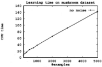
Figure 1 plots pFOIL's learning time {in CPU seconds on a Spare 1+) versus the number of examples used on the mushroom dataset from the UC/Irvine Repository. Runtime increases from about seven seconds for 100 ex amples to a little more than two minutes for 5000 ex amples; the growth is very nearly linear for the entire range. This first graph suggests that pFOIL scales up extremely well as sample sizes become large.
2.2 Reduced error pruning and noisy data
This dataset, however, is unusual in that it is virtually noise-free. 3 The situation changes radically if noise is added to the problem. To allow pFOIL to cope with noisy data, we added to pFOIL a variant of Brunk and Pazzani's reduced error pruning [1991], which was in turn inspired by Pagallo and Haussler's pruning algorithm for decision lists [1990] and earlier work in pruning decision trees [Quinlan, 1987].
The reduced error pruning algorithm consists of two phases, each of which requires an independent sample. (Practically speaking, this requires dividing the training data into two sets, a primary training set and a retrain ing set. In all the experiments of this paper, the primary training set is a random 70% and the retraining set a random 30% of the full training set.) In the first phase, which we call fitting, a rule set is found that has zero error on the primary training set. When noise is present this rule set tends to be overly complex: it "overfits"
2 The strategy of finding rule sets for each class and re solving conflicts when classifying is also used in the HYDRA system [Ali and Pazzani, 1993].
3 This can seem most easily by observing that pFOIL con verges to a hypothesis that is more than 99.95% accurate, as measured by crossvalidation on the unseen portion of the dataset .
the data. In the second phase, called simplification , a greedy strategy is used to simplify this rule set . In our implementation, two simplification operators are used: any single rule may be deleted from the rule set, or any final sequence of conditions 4 may be deleted from a rule. The reduced error pruning strategy repeatedly applies the simplification operator yielding the hypothesis with lowest error on the retraining set ; this produces a series of progressively simpler hypotheses, the error rates of which typically fall and then rise again in a U-shaped curve. The output of reduced error pruning is the hy pothesis in this series that has the lowest error rate on the retraining set .
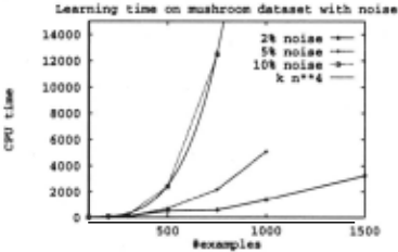
Figure 2 plots runtime versus sample size for pFOIL with reduced error pruning when 2%, 5%, and 10% clas sification noise is added to the mushroom data. The rate of growth is faster on the noisier datasets, and is always worse than linear. The curve for 10% noise, for exam ple, seems to fit the curvet= kn 4 quite well. 5 With 10% noise, pFOIL requires several hours to solve problems of relatively modest size.
We note that recent work has demonstrated that com peting learning methods-in particular decision tree in duction methods-scale quite well, even on noisy data; experiments have been performed in which tens or hun dreds of thousands of examples were used for learning [Catlett, 1991]. Unfortunately, the rapid rate of growth shown in Figure 2 makes it impractical to use rule in duction methods on large noisy datasets.
2.3 Alternative pruning methods
In this paper, we will use the implementation of reduced error pruning described above as our "strawman" noise correction method; this choice requires, perhaps, some justification. An alternative to the fit-and-simplify prun ing approach exemplified by reduced error pruning is to employ some sort of a stopping rule to keep the rule learner from overfitting the data; for example, FOIL uses an MDL-based stopping rule [Quinlan, 1990] and CN2
· For example, the rule "if w and x and y and z then class=a" might be simplified to either "if w and x and y then class=a" or "if w and x then class=a" or "if w then class=a".
5 This behavior is predicted by the analysis in Section 3.
[Clark and Niblett, 1989] uses a statistical test. However, comparative studies have shown such stopping rules to be generally inferior in the closely related problem of decision tree induction [Quinlan, 1987]; the available ev idence indicates that this also holds for rule set induction [Brunk and Pazzani, 1991].
There are also many variants of reduced error pruning; for example, Brunk and Pazzani [1991] and Pagallo and Haussler [1990] both use slightly different sets of simpli fication operators, and both choose to stop simplifying when no single simplification produces a more accurate rule set {rather than generating an entire series of rule sets and then choosing the most accurate in the series, as we do.) A more radical variation is proposed by Weiss and Indurkhya, who use a CART-like cross validation scheme to choose simplifications rather than a single re training set.
While such refinements almost certainly do have an effect on accuracy, the analysis of the next section sug gests that the time complexity of reduced error pruning is not very sensitive to the details of its implementation: in fact, the rapid growth of Figure 2 probably occurs for any fit-and-simplify greedy pruning method. In ad dition, experimental results with other systems confirm that they are also computationally expensive.
3 Understanding the problem
3.1 Complexity analysis
A complexity analysis of reduced error pruning reveals the reason for this rapid growth. In the analysis below, n denotes the number of training examples, c denotes the number of conditions in the rule set output by the fitting phase of reduced error pruning, r denotes the number of rules output in the fitting phase, d denotes the number of conditions in the rule set output by the simplify phase of reduced error pruning, and s denotes the number of rules output in the simplification phase. Also, EVAL{c, n) de notes the cost of evaluating the accuracy of a rule set with c conditions on a dataset of n examples. 6 Finally, we will assume two classes, equally represented in the training set.
With top-down separate-and-conquer rule induction systems such as pFOIL, before a condition is added to the rule set, the value of adding that condition is tested against the primary training set: in pFOIL, for exam ple, the "information gain" of the condition relative to the data is computed. The cost of testing each condition is thus proportional to the amount of relevant primary training data. A crucial point to note is that the rel evant training data includes all examples that the rule should not cover: under the assumptions above, there will be 0.1n examples in the primary data set, and at least half of these, or 0.35n examples, will be examined in adding each condition. We thus conclude that the time complexity for the fitting phase 7 is
6 ln the analysis below we will assume that this is linear in both c and n, as is the case in our implementation. It is useful to keep it separate, however, because, in some special cases-notably when rules for only a single class are learned caching techniques can be used to reduce evaluation cost. It is also possible that subsa.mpling techniques [Catlett, 1991] could be used to estimate coverage, also reducing evaluation cost.
Recall that the notation g( x) = 0{!( x)) means that g grows at least as fast as f asymptotically.
The simplification phase can be analyzed in a similar way. The outer loop, in which a single simplification is chosen, will be repeated r times in the best case. To choose a simplification our algorithm must generate e different possible simplifications, where e is the size of the last rule set (as a rule with k conditions can be sim plified in k- 1 ways, or simply deleted), and evaluate these alternative simplifications against the retraining set. Since all of the retraining set is used in each eval uation, and on the first r /2 iterations the size e of the current rule set is greater than c/2, we see that
3.2 Random data is O(n 4 )
As the experiments of Figure 2 suggest that datasets with a high rate of noise are problematic, we consider a limiting case of this: datasets which are purely random noise, with no underlying pattern whatever. Since pure noise is incompressible, the rule set output by fit must contain around n rules, each of which covers only a sin gle example. If we also assume that all attributes are binary, then each rule must have log n conditions to dis tinguish the single example that it covers from the other n examples. Thus c is roughly n log n; substituting this into Equation 1 we obtain
Substituting these values into Equation 2 we obtain
If we assume that each of the r ~ n rules in the rule sets must be tested against the data, then evaluation cost is at least rn Rj n 2 ; thus for purely random data
We draw the following conclusions from this analysis. The growth rate is unacceptably high. While the growth rate is polynomial, it is unacceptably high for an algorithm which will be used for large n.
This problem is pervasive. At first glance, it may seem that purely random incompressible data is a poor model for real-world data; however, reflection shows that this is not the case. In any data set containing a constant fraction of noisy examples, a constant fraction of the data will appear to be random incompressible noise; for instance, in the mushroom data with 5% noise added, one twentieth of the data looks like random incompressible noise. Thus almost any noisy dataset should show the same behavior in the limit; a data set that is only 5% noise would simply require twenty times the number of examples for the n 4 growth rate to be observed.
7 This argument holds for induction methods that learn DNF concepts using a. sepa.ra.te-a.nd-conquer procedure; a. similar argument, however, can be made for methods that learn decision lists.
The problem is not sensitive to the details of the imple mentation of reduced error pruning. It might be argued that our implementation does somewhat more work than is strictly necessary, and that a smaller set of simplifi cation operations (for example) might improve matters. However, let us consider a "fast" version of reduced er ror pruning which only permits entire rules to be deleted, and which stops pruning as soon as no simplification im proves the error rate. Letting s denote the number of rules output by this simplifier, for random data, the time complexity is still
Thus asymptotic time complexity is only better if r-s ~ n; in other words, performance is only improved if most of the rules which should be deleted are retained by the simplifier!
4 Improving asymptotic cost
4.1 An alternative pruning algorithm
The results indicate that a substantially different sim plification procedure is needed; they also suggest that O(n 2 ) is about the right amount of computational ef fort to expend, as faster techniques would simply lead to a learning system whose run time is dominated by the initial fitting phase. We have implemented such a pro cedure, which we call reduced error rule set re-growth.
The procedure is based on a technique used in the Grove learning system [Pagallo and Hassler, 1990]. As before, the first phase is to find a rule set Ro that overfits the primary training data. A greedy procedure is then used which starts with an emp'ty rule set and repeatedly "grows" the rule set in the manner that reduces error the most on the retraining set; this procedure stops when no growth operator reduces error. Pagallo and Haussler used a single growth operator, namely to add a single rule from Ro to the new rule set.
Pagallo and Haussler's method recovers well from un necessary rules, but behaves poorly when all of the rules learned in the fit phase contain extraneous conditions. After some experimentation, we observed that substan tially better results could be obtained with the following variant of the Pagallo and Haussler procedure, which we will call Grow . First, a rule set R0 is found by over fitting the primary data set, as before. Next, each rule ri E Ro is taken, and repeatedly simplified (using the rule simplification operator used in our implementation of reduced error pruning) in the way that either decreases its error on the primary training set the most, or, more usually, that increases its error on the primary training set the least. The result of this is a series of general izations ri,l, ... , ri,k; of the original rule ri. All of the generalizations in this series are then added to the rule set Ro .
After the initial rule set Ro has been thus expanded, we simply apply the same greedy procedure used before: starting with an empty rule set, the rule from ri,j E Ro is added which reduces error the most on the retraining set . Ties (which are not infrequent) are broken by choosing the rule that had the lowest error rate on the primary training data; if this also leads to a tie, then the smaller rule is chosen.
It can be easily shown that the time complexity of this algorithm is
where the first sum of c is the time to generalize the initial set of rules Ro. For random data, c ~ n log n, and the algorithm should generate only a small set of rules; i.e. s should be of constant size. The time complexity on random data is thus bounded by
Notice that this is asymptotically no worse than the time complexity of fitting the data.
4.2 Decreasing the cost of overfitting
The results also show that no fit-and-simplify method can do better than n 2 lo~ n, since the initial stage of overfitting can require n log n time. Thus, we have also investigated using stopping rules to prevent over fitting. Since previous research indicates that stop ping rules are usually not competitive with the fit-and simplify approach, our stopping rules are intended to be used in combination with simplification methods like Grow. In short, the goal of the stopping conditions is not to prevent overfitting entirely, but simply to reduce the amount of overfitting to more manageable levels.
We have implemented two stopping heuristics. The rule rejection heuristic examines the last rule added to a rule set, and decides whether or not to reject that rule; if the rule is rejected, then it is deleted from the rule set, and no further rules are added. Analogously, the rule specialization rejection heuristic examines a pro posed specialization of a rule being constructed, and de cides whether or not to reject the specialization; if a specialization is rejected, the learner backs up to the un specialized version of the rule, and attempts to add it to the current rule set.
Both of our heuristics are based on minimum descrip tion length principles, and require no additional training data. The basic idea in both cases is to compare the de scription length of the current rule set with an estimate of the description length of the rule set that would result by carrying through the learning process to the bitter end; for example, the rule rejection heuristic compares the description length of the current rule set with an es timate of the description length of the rule set resulting from adding enough additional rules to cover all of the remaining examples, and rejects a rule when this esti mate is much larger than the current description length. Our intention was that this very conservative stopping Benchmark Glasses Attributes Set 1
Discr Cont
audiology
20
60
iris
3
0
labor
2
8
soybean
4
35
splice
3
60
thyroid-dis
2
23
vote
2
16
t;xamples Henchmark Classes Attributes
0
4
8
0
0
6
0
226
150
57 mushroom
47
3190
3772
435
| Henchmark | Classes | Attributes | t;xamples | |
|---|---|---|---|---|
| Set 2 | Discr | Cont | ||
| bridge | 2 | 7 | 0 | 106 |
| kr-vs-kkn | 2 | 16 | 0 | 1000 |
| mushroom | 2 | 22 | 0 | 8124 |
| rds | 2 | 0 | 30 | 2500 |
| sonar | 2 | 0 | 60 | 208 |
| segment | 7 | 0 | 19 | 2310 |
| thyroid-hypo | 2 | 18 | 7 | 3163 |
| thyroid-allbp | 3 | 23 | 6 | 3772 |
criterion would improve runtime performance without adversely impacting generalization performance.
Space limitations preclude a detailed description of these heuristics. The interested reader is referred to the expanded version of this paper [Cohen, 1992b].
5 Experimental Results
To summarize, we have argued that reduced error prun ing is expensive for large, noisy datasets, and proposed two alternative techniques: a simplification algorithm that has a lower asymptotic complexity on noisy data, and an MDL-based prepruning strategy which reduces overfitting. Unfortunately, while the time complexity of the proposed simplification algorithms has been an alyzed, it is quite difficult to analyze their behavior as learning algorithms: i.e., how well the hypotheses they produce generalize the data. We thus used experimental methods to compare the performance of the proposed al gorithms. We have also experimentally tested the main predictions of the time complexity analysis.
5.1 Methodology
We assembled a set of benchmark datasets from the propositional classification-learning problems available in the UC/Irvine Repository as follows. We randomly selected seven datasets to be used for preliminary test ing, and seven to be used as a prospective test. One additional real-world dataset , which came to our notice in the final stages of testing, was added to the second group. 8 We used the first group of datasets to fine tune the Grow algorithm and the MDL pruning method; for example, the tie-breaking rules used by Grow were added after examining these datasets. However, the sec ond group of datasets were not examined during algo rithm development; i.e., all algorithms were fixed before experimentation with the second group of datasets. Thus performance on the second group can be regarded as a purely prospective test of the algorithms. The bench mark datasets are summarized in Table 1.
Our procedure for measuring error rates was also fixed before any experiments were performed: we pooled all examples and used 10-fold cross-validation [Weiss and Kulkowski, 1990] to measure accuracy. The size of the partition used for training was 90% of the total number of examples, or 500 examples, whichever was smaller; this restriction was made to prevent experimentation with reduced error pruning from being overly expensive.
8 This problem, which is labeled rds in the table, is to predict if a particular piece of switching hardware is about to enter a failure mode from various pieces of performance data. The performance data is maintained for accounting purposes and is not very good at predicting failure; thus the dataset appears quite noisy.
Many of these datasets contained missing or contin uous attributes, which pFOIL cannot handle unaided. Continuous attributes were discretized into 20 equal frequency partitions. Missing continuous attributes were replaced with the average value for that attribute; miss ing nominal attributes were replaced with the most fre quently occurring value. 9
5.2 Comparing error rates
These results are summarized in Table 2; here No Pruning represents using no pruning method, REP rep resents reduced error pruning, Grow represents our sim plification algorithm, and MDLGrow is Grow with our prepruning algorithm. Standard errors are also given; however, due to space limitations we give only summary figures for the non-prospective tests (Benchmark Set 1) . The problems are arranged in order of increasing diffi culty, as measured by the CPU time required by reduced error pruning (see Table 3), and we have highlighted the most important figures in the table: the average error rates of the three pruning algorithms on the prospec tive test. The figures indicate that Grow and MDLGrow are (at the very least) no less accurate on average than reduced error pruning. In fact, the trend is for Grow and MDLGrow to outperform reduced error pruning, al though this difference is almost never statistically signif icant for any single benchmark. 10
In performing the experiments, a few hitches arose with our proposed methodology. In two of the datasets, mushroom and kr-vs-knn, there was no noise and virtu ally no difference among the pruning methods. Thus we also considered versions of these problems (mushroom* and kr-vs-knn*) in which 10% random classification
9 An exception is the audiology dataset, which contained many attributes that were always either missing or true. For this dataset missing attributes were replaced with a special marker value. Another exception was the sonar dataset; which was discretized into only ten partitions to avoid mem ory limitations.
10 Notice also that on some datasets, every pruning method leads to a higher error rate. This may be due to noise-free data or to sparse data [Schaffer, 1992].
| Benchmark | Error rate | |||||||
|---|---|---|---|---|---|---|---|---|
| No Pruning | REP | Grow | MDLGrow | |||||
| kr-vs-lCKn | 0.1 | ± 0.03 | 0.1 | ±0.03 | 0.1 | ±0 .03 | 0.1 | ±0 .03 |
| bridge-t/d | 15.3 | 2.7 | 19.6 | 3.5 | 18.5 | 2.5 | 17.3 | 2.5 |
| thyroid-hypo | 2.3 | 0.1 | 1.6 | 0.1 | 1.5 | 0.2 | 1.5 | 0.1 |
| bridge-mtrl | 22.2 | 5.2 | 15.3 | 6.2 | 13.1 | 4.3 | 14.7 | 4.7 |
| mushroom | 0.6 | 0.1 | 1.3 | 0.3 | 1.5 | 0.2 | 1.5 | 0.2 |
| thyroid-allbp | 4.8 | 0.2 | 4.1 | 0.2 | 4.2 | 0.2 | 4.2 | 0.2 |
| bridge-span | 22.1 | 5.8 | 36.1 | 8.0 | 37.8 | 7.7 | 36.1 | 8.0 |
| bridge-rel-1 | 34.7 | 4.4 | 31.8 | 2.9 | 29.2 | 2.2 | 28.4 | 1.7 |
| bridge-type | 46.2 | 3.7 | 47.4 | 5.6 | 42.6 | 5.7 | 44.2 | 5.1 |
| sonar | 26.5 | 2.6 | 26.5 | 1.9 | 25.8 | 2.7 | 25.8 | 2.7 |
| segment | 9.6 | 0.4 | 11.9 | 0.8 | 10.8 | 0.6 | 10.8 | 0.6 |
| mushroom• | 8.2 | 0.7 | 3.6 | 0.7 | 2.8 | 0.3 | 2.9 | 0.3 |
| kr-vs-kkn• | 4.7 | 0.4 | 1.4 | 0.3 | 0.7 | 0.3 | 0.4 | 0.2 |
| rds | 30.3 | 0.4 | 29.1 | 0.7 | 29.0 | 0.5 | 24.8 | 0.4 |
| Average for Benchmark Set 2 | 17.06 | 16.43 | 15.47 | 15.19 | ||||
| Average for Benchmark Set 1 | II 9.47 | II 12.01 | 11.16 | 11.73 | ||||
6 Concluding Remarks
In this paper, we have studied the ability of rule set in duction methods to handle learning problems with many examples in the presence of noise. It was demonstrated that the best currently known method reduced error . ' prunmg, requires large amounts of time to handle large datasets: asymptotically, the complexity of the method grows as n 4 for noisy datasets of n examples. Two solu tions to this problem were proposed. First, an alterna tive pruning method that requires only time proportional to n 2 log n was described. In spite of its asymptotically faster performance, this method finds hypotheses that are at least as accurate as those found by reduced error pruning; in fact, it outperforms reduced error pruning on seventeen of twenty-one benchmark problems. The second technique for dealing with the high cost of prun in~ was a .prepruning method based on MDL principles; th1s techmque was also shown to reduce runtime without leading to any degradation in classification accuracy.
The techniques described in this paper appear to ex tend easily to relational learning problems; however, this
noise was added to the training data. Also on closer . . ' exammat10n, the bridge dataset turned out to contain five different classification problems, as it contained five different dependent attributes which needed to be pre dicted. We include results for all of the five bridge prob lems. This perhaps weights the average results some what too heavily to pruning methods that do well on this dataset; however, if the five bridge problems are weighted as a single problem, the results are qualitatively the same. The results are also qualitatively the same if the mushroom· and kr-vs-knn* benchmarks, which con tain artificial noise, are omitted. 11
5.3 Comparing time complexity
Table 3 shows the corresponding results for CPU time. To summarize, Grow and REP are comparable for benchmarks that are either small in size or free of noise; similarly, MDLGrow is comparable to Grow on smaller problems. On larger problems, however, Grow is ~uch fast~r than reduced error pruning, and MDLGrow 1s faster stlll; many of these differences are highly statis tically significant. On average, MDLGrow is more than ten times faster in the prospective test.
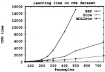
We also undertook somewhat more detailed studies of CPU time performance on selected benchmarks. Fig ~re 3 ~h~ws the results for the rds dataset, which is typ ~cal (s1m1lar results fo~ three other benchmarks are given m the expanded versiOn of this paper [Cohen, 1992b].) These results serve as additional confirmation of the main claim of the paper: that the runtime of Grow and MDLGrow is asymptotically faster than reduced error pruning.
11 '_Veighting the bridge problems as one, the average error rate IS 10.97% for reduced error pruning, 10.37% for Grow, and 10.02% for MDLGrow. If one also discounts the artificial problems, the average error rate is 13.09% for reduced error pruning, 12.52% for Grow, and 12.11% for Grow with MDL pruning.
| Benchmark | CPU T1me | |||||||
|---|---|---|---|---|---|---|---|---|
| No Pruning | REP | Grow | MDLGrow | |||||
| kr-vs-kkn | 10.8 | ± 0.6 | 18.5 | ±1.8 | 13.2 | ±0 .6 | 13.4 | ±0.6 |
| bridge-t/d | 12.7 | 0.9 | 27.6 | 3.3 | 10.4 | 0.9 | 8.1 | 0.7 |
| thyroid-hypo | 72.6 | 6.5 | 56.6 | 9.4 | 46.4 | 6.2 | 48.1 | 6.3 |
| bridge-mtrl | 22.1 | 0.6 | 76.7 | 9.6 | 16.5 | 1.5 | 10.6 | 0.6 |
| mushroom | 35.6 | 0.8 | 78.3 | 7.8 | 44.5 | 1.4 | 45.3 | 1.7 |
| thyroid-allbp | 144.8 | 7.7 | 164.5 | 12.6 | 99.5 | 4.6 | 100.7 | 5.8 |
| bridge-span | 29.5 | 0.8 | 176.2 | 18.6 | 31.9 | 2.3 | 13.3 | 0.8 |
| bridge-rel-1 | 44.1 | 1.0 | 294.1 | 36.9 | 34.0 | 2.9 | 14.1 | 1.2 |
| bridge-type | 38.9 | 1.1 | 370.6 | 25.2 | 40.5 | 2.3 | 21.2 | 1.0 |
| sonar | 561.0 | 12.9 | 399.2 | 15.1 | 368.2 | 12.0 | 370.6 | 12.1 |
| segment | 815.7 | 23.9 | 1264.0 | 86.6 | 728.2 | 29.6 | 733.6 | 27.8 |
| mushroom* | 217.2 | 10.1 | 4081.7 | 485.4 | 276.7 | 23.4 | 135.1 | 6.9 |
| kr-vs-kkn* | 154.2 | 11.9 | 5549.3 | 1255.3 | 206.6 | 23.5 | 53.5 | 4.0 |
| rds | 3189.1 | 84.9 | 15155.2 | 1282.4 | 2210.0 | 52.0 | 879.9 | 42.4 |
| Average for Benchmark Set 2 | 382.03 | 2695.63 | 402.00 | 239.38 | ||||
| I Average for Benchmark Set 1 | II 108.4 | 384.0 | 105.9 | 100.5 | ||||
still needs to be verified experimentally. (The MDL based prepruning, for example, may need modification to work properly on relational problems.) Also, while the techniques described here have natural extensions which can be applied in learnin$ from examples and a grammatical bias [Cohen, 1992aj, these extensions have again not been experimented with systematically.
Acknowledgments.
Many thanks to Jason Catlett, Haym Hirsh, and Mike Pazzani for comments on an early draft of this paper, to Susan Cohen for proofreading it, and to Wan-Ping Chiang for providing the rds data.
@inproceedings{ijcai1993p136,
  title     = {Efficient Pruning Methods for Separate-and-Conquer Rule Learning Systems},
  author    = {Cohen, William W.},
  booktitle = {Proceedings of the Thirteenth International Joint Conference on
               Artificial Intelligence, {IJCAI-93}},
  publisher = {International Joint Conferences on Artificial Intelligence},
  editor    = {Ruzena Bajcsy},
  pages     = {988--993},
  year      = {1993},
  note      = {Machine Learning},
  url       = {https://ijcai.org/proceedings/1993/136},
}
TY - CPAPER TI - Efficient Pruning Methods for Separate-and-Conquer Rule Learning Systems AU - Cohen, William W. T2 - Proceedings of the Thirteenth International Joint Conference on Artificial Intelligence, IJCAI-93 PB - International Joint Conferences on Artificial Intelligence PY - 1993 SP - 988 EP - 993 UR - https://ijcai.org/proceedings/1993/136 ER -Copied
Machine-readable versions of this paper, for tools and AI agents:





