
Bayesian Classification with Correlation and Inheritance
Proceedings of the Twelfth International Joint Conference on Artificial Intelligence. Learning Be Knowledge Acquisition. Pages 692-697.
© 1991 International Joint Conferences on Artificial Intelligence
Abstract
The task of inferring a set of classes and class descriptions most likely to explain a given data set can be placed on a firm theoretical foundation using Bayesian statistics. Within this framework, and using various mathematical and algorithmic approximations, the AutoClass system searches for the most probable classifications, automatically choosing the number of classes and complexity of class descriptions. Simpler versions of AutoClass have been applied to many large real data sets, have discovered new independently-verified phenomena, and have been released as a robust software package. Recent extensions allow attributes to be selectively correlated within particular classes, and allow classes to inherit, or share, model parameters though a class hierarchy.
- [Berger, 1985] J. 0. Berger. Statistical Decision Theory and Bayesian Analysis. Springer-Verlag, New York, 1985.
- [Cheeseman et al., 1988a] P. Cheeseman, J. Kelly, M. Self, J. Stutz, W. Taylor, and D. Free- man. Autoclass: a Bayesian classification system. In Proceedings of the Fifth International Conference on Machine Learning, 1988.
- [Cheeseman et al., 1988b] P. Cheeseman, M. Self, J. Kelly, J. Stutz, W. Taylor, and D. Freeman. Bayesian classification. In Seventh National Conference on Artificial Intelligence, pages 607-611, Saint Paul, Minnesota, 1988.
- [Dempster et al., 1977] A.P. Dempster, N.M. Laird, and D.B. Rubin. Maximum likelihood from incomplete data via the EM algorithm. J. Roy. Statist. Soc. B, 39:1-38, 1977.
- [D.M.Titterington et al., 1985] D.M.Titterington, A.F.M. Smith, and U.E. Makov. Statistical Analysis of Finite Mixture Distributions. John Wiley & Sons, New York, 1985.
- [Goebel et al., 1989] J. Goebel, K. Volk, H. Walker, F. Gerbault, P. Cheeseman, M. Self, J. Stutz, and W. Taylor. A Bayesian classification of the IRAS LRS atlas. Astron. Astrophys., 222:L5-L8, 1989.
- [Hanson et al., 1991] Robin Hanson, John Stutz, and Peter Cheeseman. Bayesian classification theory. Technical Report FIA-90-12-7-01, NASA Ames Re- search Center, Artificial Intelligence Branch, 1991.
- [Hunter and States, 1991] Lawrence Hunter and David States. Applying Bayesian classification to protein structure. In IEEE Conference on Applications of AI, 1991.
- [Mardia et al., 1979] K.V. Mardia, J.T. Kent, and J.M. Bibby. Multivariate Analysis. Academic Press Inc., New York, 1979.
- [Spiegel, 1968] Murray Spiegel. Mathematical Handbook of Formulas and Tables. McGraw-Hill Book Company, New York, 1968.
References were extracted automatically from the PDF and may contain errors.
Full text extracted automatically from the PDF; figures, tables and equations may differ. The PDF is the version of record.
1 Introduction
The task of supervised classification- i.e., learning to pre dict class memberships of test cases given labeled train ing cases - is a familiar machine learning problem. A re lated problem is unsupervised classification, where train ing cases are also unlabeled. Here one tries to predict all features of new cases; the best classification is the least "surprised" by new cases. This type of classification, related to clustering, is often very useful in exploratory data analysis, where one has few preconceptions about what structures new data may hold.
We have previously developed and reported on Au toClass [Cheeseman et al., 1988a; Cheeseman et al., 1988b], an unsupervised classification system based on Bayesian theory. Rather than just partitioning cases, as most clustering techniques do, the Bayesian approach searches in a model space for the "best" class descrip tions. A best classification optimally trades off predic tive accuracy against the complexity of the classes, and so does not "overfit" the data. Such classes are also "fuzzy"; instead of each case being assigned to a class, a case has a probability of being a member of each of the different classes.
·Research Institute for Advanced Computer Science
Autoclass III the most recent released version, com-' . hines real and discrete data, allows some data to be IlllSSing, and automatically chooses the ~umber ~f ~lasses from first principles. Extensive testmg has md1cated that it generally produces significant and useful results, but is primarily limited by the simplicity of the mod els it uses, rather than, for example, inadequ~te search heuristics. AutoClass III assumes that all attnbutes are relevant that they are independent of each other within each cl~, and that classes are mutually exclusive. Re cent extensions, embodied in Autoclass IV, let us relax two of these assumptions, allowing attributes to be se lectively correlated and to have more or less relevance via a class hierarchy.
We begin by describing the Bayesian theory of learn ing, and then apply it to increasingly complex classifi cation problems, from various single class models up to hierarchical class mixtures. Finally, we report empirical results from an implementation of these extensions.
2 Bayesian Learning
Bayesian theory gives a mathematical calculus of degrees of belief, describing what it means for beliefs to be con sistent and how they should change with evidence. This section briefly reviews that theory, describes an approach to making it tractable, and comments on the resulting tradeoffs. In general, a Bayesian agent uses a single real number to describe its degree of belief in each proposi tion of interest.
2.1 Theory
Let E denote some evidence that is known or could po tentially be known to an agent; let H denote a hypothesis specifying that the world is in some particular state; and let the sets of possible evidence E and possible states of the world H each be mutually exclusive and exhaustive sets.
In general, P(abicd) denotes a real number describing an agent's degree of belief in the conjunction of proposi tions a and b, conditional on the assumption that propo sitions c and d are true. More specifically, 1r(H) is a "prior" describing the agent's belief in H before, or in the absence of, seeing evidence E, 1r(HIE) is a "poste rior" describing the agent's belief after observing some particular evidence E, and L(EIH) is a "likelihood" em-
Peter Cheeseman ruAcs·
bodying the agent's theory of how likely it would be to see each possible evidence combination E in each possi ble world H.
To be consistent, beliefs must be non-negative, P(aib);::: 0, and normalized, so that L:H 1r(H) = 1 and L:E L(EIH) = 1. The likelihood and the prior together give a "joint" probability J(EH)::: L(EjH)1r(H) ofboth E and H. Normalizing the joint gives Bayes' rule, which tells how beliefs should change with evidence.
When the set of possible Hs is continuous, the prior 1r(H) becomes a differential d1r(H), and the sums over H are replaced by integrals. Similarly, continuous Es have a differential likelihood dL(EiH), though any real evidence ll.E will have a finite probability ll.L(EiH) ~ dL(EiH)~:.
In theory, all an agent needs to do in any given situa tion is to choose a set of states H, an associated likelihood function describing what evidence is expected to be ob served in those states, a set of prior expectations on the states, and then collect some evidence. Bayes' rule then specifies the appropriate posterior beliefs about the state of the world, which can be used to answer most questions of interest.
2.2 Practice
In practice this theory can be difficult to apply, as the sums and integrals involved are often mathematically in tractable. Here is our approach.
Rather than consider all possible states of the world, we focus on some smaller space of models, and do all of our analysis conditional on an assumption S that the world really is described by one of the models in our space. This assumption is almost certainly false, but it makes the analysis tractable.
The parameters which specify a particular model are split into two sets. First, a set of discrete parameters T describe the general form of the model, usually by spec ifying some functional form for the likelihood function. For example, T might specify whether two variables are correlated or not, or how many classes are present in a classification. Second, free variables in this general form, such as the magnitude of the correlation or the relative sizes of the classes, constitute the remaining continuous model parameters V.
We generally prefer a likelihood 1 L(EIVTS) which is mathematically simple and yet still embodies the kinds of complexity relevant in some context.
Similarly, we prefer a simple prior distribution d1r(VTjS) over the model space, allowing the resulting V integrals, described below, to be at least approximated. We also usually prefer a relatively broad and uninfor mative prior, and one that gives nearly equal weight to different levels of model complexity, resulting in a "sig nificance test". Adding more parameters to a model then induces a cost, which must be paid for by a significantly better fit to the data before the more complex model can be preferred.
1 A variable like V in a probability expression stands for the proposition that the variable has a particular value.
The joint can now be written as dJ(EVTIS) = L(EIVTS) d1r(VTjS) and, for a reasonably-complex problem, is usually a very rugged distribution in VT, with an immense number of sharp peaks distributed widely over a huge high-dimensional space. Because of this we despair of directly normalizing the joint, as re quired by Bayes' rule, or of communicating the detailed shape of the posterior distribution.
Instead we break the continuous V space into regions R surrounding each sharp peak, and search until we tire for combinations RT for which the "marginal" joint
is as large as possible. The best few such "models" RT found are then reported, even though it is usually almost certain that more probable models remain to be found.
Each model RT is reported by describing its marginal joint M(ERTIS), its discrete parameters T, and esti mates of typical values of V in the region R, such as the mean estimate of V:
or the V for which dJ(EVTIS) is maximum in R. While these estimates are not invariant under reparameteriza tions of the V space, and hence depend on the syntax with which the likelihood was expressed, the peak is usu ally sharp enough that such differences don't matter.
A weighted average of the best few models found is used to make predictions. Almost all of the weight is usually in the best few, justifying the neglect of the rest.
Even though the sums and integrals can be difficult, and large spaces must be searched, Bayesian theory offers the advantages of being theoretically well-founded and empirically well-tested [Berger, 1985]; one can almost "turn the crank", modulo doing integrals and search 2 , to deal with any new problem. Disadvantages include being forced to be explicit about the space of models one is searching in, and occasional ambiguities regarding what an appropriate prior is. Also, it is not clear how one can take the computational cost of doing a Bayesian analysis into account without a crippling infinite regress.
We will now illustrate this general approach by apply ing it to the problem of unsupervised classification.
3 Single Class Models
For all the models to be considered in this paper, the evidence E will consist of a set of I cases, an associated set JC of attributes, of size 3 K, and case attribute values 4
2 The joint probability provides a good local evaluation function for searching though.
3 We use script letters like 1C to denote sets, and matching ordinary letters K to denote their size.
4 Nothing in principle prevents a Bayesian analysis of more complex model spaces for relational data.
X;k, which can include "unknown." 5 For example, med ical case number 8, described as (age = 23, blood-type= A, ... ), would have Xs,t = 23, Xs,2 = A, etc.
In this section and the next we will describe appli cations of Bayesian learning theory to various kinds of models which could explain this evidence, beginning with simple model spaces and building more complex spaces from them. We begin in this section with a sin gle class. First, a single attribute is considered, then multiple independent attributes, then fully covariant at tributes, and finally selective covariance. In the next section we combine these single classes into class mix tures, first flat then tree-based.
| Space | Description | v | T | R |
| SDl | Smgle Discrete | q, | ||
| SRt | Single Real | JJ.<T | ||
| Sr | Independent Attrs | vk | ||
| Sv | Covariant Discrete | q,l,2··· | ||
| SR | Covariant Real | Ji.k:Ekk 1 | ||
| Sv | Block Covariance | vb | Bleb | |
| SM | Flat Class Mixture | ac Vc | c | R |
| SH | Tree Class Mixture | acVc | JclCcTc | R |
For each space S we will describe the continuous pa rameters V, any discrete model parameters T, normal ized likelihoods L(EIVTS), and priors 11'(VTIS). As most spaces have no discrete parameters T, and only one region R, we can usually ignore these parameters. Ap proximations to the resulting marginals M(ERTIS) and estimates £(VIERTS) will be given, but not derived. These will often be given in terms of general functions F which are common to various models. As appropriate, comments will be made about algorithms and computa tional complexity.
All of the likelihood functions considered here as sume the cases are independent, i.e., L(EIVTS) = Il; L(E;IVTS) so we need only give L(E;IVTS) for each space, where E; = {X;t,Xi2·····X;K}·
4 Single Class Models
4.1 Single Discrete Attribute- SDl
A discrete attribute k allows only a finite number of possible values 1 E [1, 2, ... , L] for any X;. A set of in dependent coin tosses, for example, might have L = 3 with It = heads, 12 = tails, and 13 = "unknown". If we make the assumption Sv1 that there is only one discrete attribute, then the only parameters are the continuous V = q1 ... qL consisting of the likelihoods L(X;IVSDl) = q(l=X;) for each possible value I. In the coin example, q1 = . 7 would say that the coin had a 70% of coming up heads each time.
6 H the fact that a data value is unknown might be infor mative, one can model "unknown" as just another possible (discrete) data value; otherwise the likelihood for an unknown value is just a sum over the possible known values.
There are only L - 1 free parameters since normal ization requires 2: 1 q, = 1. For this likelihood, all that matters from the data for the total L(EIVTSdt) are the number of cases with each value 6 I1 = 2:; 6x, 1· In the coin example, I 1 would be the number of heads. Such sums are called "sufficient statistics" since they summa rize all the information relevant to a model.
We choose a prior 7
which for a > 0 is a special case of a beta distribution [Berger, 1985]. a is a "hyperparameter" which can be set to different values to specify different priors. ·Here we set a = 1/ L. This simple problem has only one maximum, whose marginal is given by
The prior above was chosen because it scales nicely, and to simplify the mean estimate of q,
for a = 1/ L. Using a hash table, these results can be computed in order I numerical steps, independent of L.
4.2 Single Real Attribute- SRt
Real attribute values X; specify a small range of the real line, with a center x; and a precision, Llx;, assumed to be much smaller than other scales of interest. For example, someone's weight might be measured as 70±1 kilograms.
For SRl, where there is only one real attribute, we assume the likelihood is a standard normal distribu tion, where the sufficient statistics are the data mean x = J I:[ x;, the geometric mean precision & = (IJ{Llx;)t and the standard deviation s given by s 2 = .! L:;(x;- x) 2 · V consists of a model mean J1. and stan clard deviation a. For example, people's weight might be distributeds with a mean of 80 kilograms and a deviation of 15.
For brevity we here give only the resulting marginal
where LlJJ. = max x; - minx;, and estimates, which are simply £(JJ.IESRt) = x, and £(alE) = j;i;;s. See [Hanson et al., 1991] for more details. Computation here takes order I steps, used to compute the sufficient statis tics.
4.3 Independent Attributes - S1
We now introduce some notation for collecting sets of indexed terms like X;k. A single such term inside a {} will denote the set of all such indexed terms collected across all of the indices, like i and k in E = { X;k} ::: {X;k such that i E [1, ... , I], k E A:}. To collect across only some of the indices we use Uk as in E; = Uk X;k ::: {Xil, X;2, ... }, all the evidence for a single case i.
6 Don denotes 1 when u = 11 and 0 otherwise.
7 f(y) is the Gamma function [Spiegel, 1968].
8 Actually, log( weight) is more normally distributed.
The simplest way to deal with cases having multiple attributes is to assume S1 that they are all independent, i.e., treating each attribute as if it were a separate prob lem. In this case, the parameter set V partitions into parameter sets vk = u,~ q,~ or (J.lk, O'k], depending on whether that k is discrete or real. The likelihood, prior, and joint for multiple attributes are all simple products of the results above for one attribute: s1 = SD1 or SR1- i.e., L(E;IVSI) = flk L(X;kiVkSi), d1r(VIS1) = TI" d1r(VkiS1), and M(EIS1) = fl" M(E(k)ISl) where E(k) = U; X;k, all the evidence associated with at tribute k. The estimates e(VkiES1) = e(VkiE(k)Sl) are exactly the same. Computation takes order I K steps here.
4.4 Fully Covariant Discretes - S D
A model space SD which allows a set A: of discrete attributes to fully covary (i.e, contribute to a likeli hood in non-trivial combinations) can be obtained by treating all combinations of base attribute values as particular values of one super attribute, which then has L' = flk Lk values 9 V consists of terms like q,z, .. .zK, indexed by all the attributes. I 1 generalizes to I,l,2 ···'K = L:; nk 6"'·~'~. Given this transformation, the likelihoods, etc. look the same as before: L(E; I VSD) = qz 1 12 ··· 1K' where each lk = X;k, d1r(VISD) = dB( {q,l,2···'K} I L'), M(EISD) = F1( {I,l,2··.lK} 'I, L'), and 10 e(qlll, .. .lK IESD) = F2(I,l,2·· .lK' I, L') Computa tion takes order I K steps here. This model could, for example, use a single combined hair-color eye-color at tribute to allow a correlation between people being blond and blue-eyed.
4.5 Fully Covariant Reals- SR
If we assume SR that a set A: of real-valued attributes follow the standard multivariate normal distribution, we replace the 0'~ above with a model covariance ma trix ~kk' and 8~ with a data covariance matrix skk' = f L:;(X;k - Xk)(xik' - Xk' ). The inverse Wishart distri bution [Mardia et al., 1979] gives an integrable prior on :Ekk'· We again give only the marginal joint 11
and estimates 12
9 L' can be a very large number!
1 ° F1 and F2 are defined in Section 4.1.
11 At present, we lack a satisfactory way to approximate this marginal when some values are unknown.
12 To obtain these formulas, certain free hyperparameters in the Wishart prior have been set using simple statistics from the data. This is more robust and simplifies the math, but is "cheating" because priors are supposed to be independent of the data. Similar cheating was also done in Section 4.2.
E(~H·IESR) = 1 j~·t Sw. See [Hanson et al. , 1991] for details. Computation here takes order (I+ K)K 2 steps.
4.6 Block Covariance - Sv
Rather than just having either full independence or full dependence of attributes, we prefer a model space Sv where some combinations of attributes may covary while others remain independent, with full or no dependence as special limiting cases. This allows us to avoid paying the cost of specifying covariance parameters when they cannot buy us a significantly better fit to the data.
Our approach to partial dependence is simply to par tition the attributes A: into B blocks A:b, each of size Kb, with full covariance within each block and full indepen dence between blocks. 13 We also currently prohibit reals and discretes in the same covariant block.
The evidence E partitions block-wise into E(A:b) (using E;(A) ::: U" ..tX;" and E(A) ::: {E;(A)}), each with its own suftfcient statistics; and the param eters V partition into parameters ~ = {qz 1 z 2 ··· lK} or [{:Ekk'}, {J.'k}]. Each block is treated as a different problem, except that we now also have discrete param eters T = [B, {A:b}] to specify. Thus the likelihood L(E;jVTSv) = fl~ L(E;(A:b)I~Ss) is a simple product of block terms Ss = SD or SR assuming full covariance within each block, and the estimates e(VbiETSv ) = e(VbiE(A:b)Ss) are the same as before.
We choose a prior d?r(VTISv) = 1!'( B { A:b} ISv) nb d?r(~ IS B) which predicts the block structure B {A:b} independently of the parameters vb within each independent block result ing in a similarly decomposed marginal M(ETISv) = ?r(B{A:b}ISv)flbM(E(A:b)ISs). We choose a block structure prior
where A:R is the set of real attributes and BR is the number of real blocks (and similarly for A:D and BD ). It is normalized using Z(A, U) ::: '\'u ( 1 )u-1 (U-u+l)A L...tu=1 - (u u+l)! (u 1)! , the number of ways one can partition a set with A elements into U subsets. This prior prefers the special cases of full covariance and full independence, and thus includes a significance test. For example, in comparing the hypothesis that each at tribute is in a separate block (i.e., all independent) with the hypothesis that only one particular pair of attributes covary together in a block of size two, this prior penalizes the covariance hypothesis in proportion to the number of such pairs possible.
Computation here takes order NK(IKb + Kl) steps, where N is the number of search trials done before quit ting, which would be around (K- 1)! for a complete search of the space. Kb is an average, over both the search trials and the attributes, of the block size of real attributes (and unity for discrete attributes).
13 We choose it because it is easy, fits well with our model of class hierarchy, and allows full dependence.
5 Class Mixtures
5.1 Flat Mixtures - SM
The above model spaces Sc = Sv or 81 can be thought of as describing a single class, and so can be extended by considering a space S M of simple mixtures of such classes [D.M.Titterington et al., 1985]. With Sc = 81, this is the model space of AutoClass III, and Figure 1 shows how it can fit a set of artificial real-valued data in five dimensions.
In this model space the likelihood L(E;IVTSM) = 2::; acL(E;IV.:TcSc) sums over products of "class weights" ac, each giving the probability that any case would belong to class c of the C classes, and class like lihoods describing how members of each class are dis tributed. In the limit of large C this model space is gen eral enough to be able to fit any distribution arbitrarily closely, and hence is "asymtotically correct".
The parameters T = [C, {Tc}] and V = [{ac}, {V.,}] combine parameters for each class and parameters de scribing the mixture. The prior is similarly broken down
where F3(C) = 2~2 for C > O.The ac is treated as if the choice of clCU: were another discrete attribute, except that a C! is added because classes are not distinguishable a priori.
Except in very simple problems, the resulting joint dJ(EVTIS) has many local maxima, and so we must now distinguish regions R of the V space. To find a local maxima we use the "EM" algorithm [Dempster et al., 1977] which is based on the fact that at a maxima the class parameters V., can be estimated from weighted sufficient statistics. Relative likelihood weights Wic = acL(E;IV.:TcSc)/L(E;IVTSM), satisfying Ecwic = 1 give the probability that a particular case i is a member of class c. Using these weights we can break each case into "fractional cases", assign these to their respective classes, and create new "class data" Ec = Uik [X;~;, w;c] with new weighted class sufficient statistics obtained by using weighted sums 2::; Wic instead of sums 2::;· For ex ample Ic = 2::; Wic and Xkc = L 2::; W;cXik· Substituting these statistics into any previous class likelihood function L(EIV.:TcSc) gives a weighted likelihood L'(EciV.:TcSc) and associated new estimates and marginals.
At the maxima, the weights Wic should be consistent with estimates of V = {[ac, Cc]} from e(V.,IERSM) = e'(V.,IEcSc) and e(aciERSM) = F2(Ic,I, C). To reach a maxima we start out at a random seed and repeatedly use our current best estimates of V to compute the w;c, and then use the Wic to re-estimate the V, stopping after 10 - 100 iterations when they both predict each other.
Integrating the joint in R can't be done directly be cause the product of a sum in the full likelihood is hard to decompose, but by using fractional cases to approxi mate the likelihood L(E;IVTRSm) =
while holding the Wic fixed, we get an approximate marginal:
Our standard search procedure begins each converging trial from classes built around C random case pairs. The number of classes C is chosen randomly from a log normal distribution fit to the Cs of the 6- 10 best trials seen so far, after trying a fixed range of Cs to start. We also have developed alternative search procedures which selectively merge and split classes according to various heuristics. While these usually do better, they some times do much worse.
The marginal joints of the different trials generally follow a log-normal distribution, allowing us to estimate during the search how much longer it will take on average to find a better peak, and how much better it is likely to be.
In the simpler model ~ace SMI where Sc = 81 the computation is order NICK, where C averages over the search trials. N is the number of possible peaks, out of the immense number usually present, that a compu tation actually examines. ·In the covariant space SMv where Sc = Sv this becomes NKC(IKb + Kc).
5.2 Class Hierarchy and Inheritance- SH
When there are many attributes and each class must have its own set of parameters for each of these at tributes, multiple classes are strongly penalized. At tributes which are irrelevant to the whole classification, like a medical patient's favorite color, can be particularly costly. To reduce this cost, one can allow classes to share the specification of parameters associated with some of their independent blocks.
Rather than allow arbitrary combinations of classes to share blocks, it is simpler to organize the classes as leaves of a tree. Each block can be placed at some node in this tree, to be shared by all the leaves below (far ther from the root than) that node. In this way different attributes can be explained at different levels of an ab straction hierarchy. For medical patients the tree might have viral-infections near the root, predicting fevers, and some more specific viral disease near the leaves, predict ing more disease specific symptoms. Irrelevant attributes like favorite-color would go at the root. To make predic tions about a member of a leaf class, one first inherits down the attribute descriptions from classes above it.
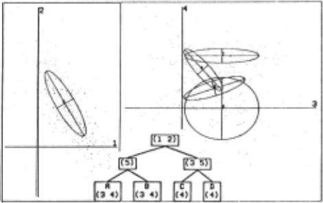
Therefore the above class mixture model space SM can be generalized to a hierarchical space S H by replacing the above set of classes with a tree of classes, and using the tree to inherit specifications of class parameters. From the view of the parameters specified at a class, all of the classes below that class pool their weight into one big class. Figure 3 shows some sample trees, and Figure 2 shows how a class tree, this time with Sc = Sv, can better fit the same data as in Figure 1.
A tree of classes has one root class r. Every other class c has one parent class Pc, and every class has Jc child classes given by Cc;, where the index j ranges over the children of a class. Each child class has a weight CXcj relative to its siblings, with ~Jc CXcj = 1, and an absolute weight ClCcj = ClcjClc 1 With Clr = 1.
Each class has an associated set of attributes K-c, which it predicts independently through a likelihood L(Ei(X:.c)IVcTcSc) and which no class above or below it predicts. To avoid having redundant trees which describe the same likelihood function, only K-r can be empty, and non-leaves must have Jc 2: 2.
We need to ensure that all attributes are predicted somewhere at or above each leaf class. So we call Ac the set of attributes which are predicted at or below each class, start with A,. = K, and then recursively par tition each Ac into attributes K-c "kept" at that class, and hence predicted directly by it, and the remaining attributes to be predicted at or below each child AccJ. For leaves Ac = K-c.
Expressed in terms of the leaves the likelihood is again a mixture L(EiiVTSM) =
allowing the same EM procedure as before to find local maximas. The case weights here Wei = ~Jc wccJi (with Wri = 1) sum like in the flat mixture case and define class statistics EC(X:.c) = ukEKc,i [Xik, Wei]·
We also choose a similar prior, though it must now specify the K-c as well: d1r(VTISH) =
for all subsets K-c of Ac of size in the range [1- Ccr 1 Ac], except that F3(Jc -1) is replaced by Cole when Ac = K-c. Note that this prior is recursive, as the prior for each class depends on the what attributes have been chosen for its parent class.
This prior says that each possible number of attributes kept is equally likely, and gi..;en the number to be kept each particular combination is equally likely. This prior prefers the simpler cases of K-c = Ac and Kc = 1 and so again offers a significance test. In comparing the hy pothesis that all attributes are kept at a class with the hypothesis that all but one particular attribute is kept at that class, this prior penalizes the all-but-one hypothe sis in proportion to the number of attributes that could have been kept instead.
The marginal joint becomes M(ERTISH) ~
Searching in this most complex space SHv is challeng ing. There are a great many search dimensions where one can trade off simplicity and fit to the data, and we have only begun to explore possible heuristics. Blocks can be merged or split, classes can be merged or split, blocks can be promoted or demoted in the class tree, EM itera tions can be continued farther, and one can try a random restart to seek a new peak. But even the simplest ap proaches to searching a more general model space seem to do better than smarter searches of simpler spaces.
6 Results
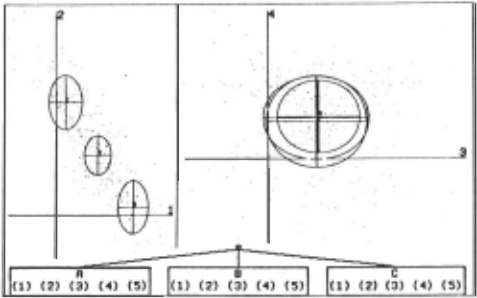
We plot attributes 1 vs. 2, and 3 vs. 4 for an artificial data set. One u deviation ovals are drawn around the centers of the three classes.
and estimates are e(VciERS{I) = .e'(Vc IEc(X:.c)Sc) and e(ac;IERSH) = Fz(Ic;, Ic.JcJ agam.
In the general case of SHv, where Sc = Sv, computation again takes N KC(IKb + KC), except that the J is now also an average of, for each k, the number of classes in the hierarchy which use that k (i.e., have k E K-c)· Since this is usually less than the number of leaves, the model SH is typically cheaper to compute than SM for the same number of leaves.
We have built a robust software package, AutoClass III, around the flat independent model SMI, with utilities for reading data, controlling search, and viewing results, and have released it for general use. It is written in Com monLisp, and runs on many different machines. We, and others, have applied this system to many large and real databases. When applied to infrared stellar data we found new, independently verified, phenomena [Goebel et al., 1989]. Others have successfully applied it to pro tein structure [Hunter and States, 1991].
We are now developing Autoclass IV around the full hierarchical block covariant model space S HV. As hoped, it gives a significant improvement over the previous ver sion when applied to real data, though we have only tried it on small problems so far. On the standard IRJS flowers data (150 cases, 4 attributes) we find a model over 10 6 s times more probable than the independent model, i.e., with a marginal joint (absolute value 10- 913 ) that much larger . 14 This compares with typical improvements of 10 2 for doubling the search time or for using a smarter merging search.
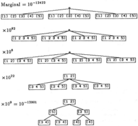
each new class tree.
Figures 1, 2, and 3 illustrate a similar gain on an artifi cial data set with 400 cases and 5 real attributes. Figure 1 shows how the data is distributed in attributes #1 and #2, and in attributes #3 and #4 (attribute #5 is not shown). Superimposed upon this is the best result found with Autoclass III.
Since the data is dominated by a covariance between attributes #1 and #2, the independent model tries to model this by stringing classes along the 1 - 2 covari ance axis. There is too little data to justify any more structure in this model class, so the #3, #4 and #5 axes are basically ignored. The
Figure 3 shows a progression of models between this model and the current best answer from Autoclass IV, given in Figure 2. Each new model adding one new fea ture and gains an improved marginal joint. Moving from a flat independent model to a flat fully covariant model, the best model found is over 10 81 times more probable, with 4 classes each of which have significant covariances in 2 pairs of attributes. This large gain comes from com bining a much better fit to the data, despite extra costs paid for the added class and covariance parameters. But, on inspection one finds that the four covariant classes are virtually the same in the 1 - 2 projection and show little correlation with the other attributes. We therefore split the covariance blocks and raise the (1 2) block to the common root for another relative increase of 10 30 · This process can be repeated on pairs of the (3 4 5) blocks to get the 3 level tree shown in Figure 2, gaining another 10 9 in relative probability. We have thus gained a to tal factor of over 10 120 in relative marginal probability over the best classification found using the independent model. Of that total, about 10 39 comes from the fact that the tree now requires fewer parameters to specify a similar likelihood.
14 Cross-validation would probably be a better test here, since our priors are fairly crude.
These preliminary results support previous indications that the ability to represent various kinds of structures in the data is the major limiting factor of such a system.
@inproceedings{ijcai1991p101,
  title     = {Bayesian Classification with Correlation and Inheritance},
  author    = {Hanson, Robin and Stutz, John C. and Cheeseman, Peter C.},
  booktitle = {Proceedings of the Twelfth International Joint Conference on
               Artificial Intelligence, {IJCAI-91}},
  publisher = {International Joint Conferences on Artificial Intelligence},
  editor    = {John Mylopoulos and Ray Reiter},
  pages     = {692--697},
  year      = {1991},
  month     = {8},
  note      = {Learning Be Knowledge Acquisition},
  url       = {https://ijcai.org/proceedings/1991/101},
}
TY - CPAPER TI - Bayesian Classification with Correlation and Inheritance AU - Hanson, Robin AU - Stutz, John C. AU - Cheeseman, Peter C. T2 - Proceedings of the Twelfth International Joint Conference on Artificial Intelligence, IJCAI-91 PB - International Joint Conferences on Artificial Intelligence PY - 1991 SP - 692 EP - 697 UR - https://ijcai.org/proceedings/1991/101 ER -Copied
Machine-readable versions of this paper, for tools and AI agents:





