Single-Agent Parallel Window Search: A Summary of Results

1 Introduction and Overview

Heuristic search is a fundamental problem-solving method in artificial intelligence. Common examples of single-agent search problems are the Eight Puzzle and its larger relative the Fifteen Puzzle. The Eight Puzzle con­ sists of a 3x3 square frame containing 8 numbered square tiles and an empty position called the 'blank'. The legal operators slide any tile horizontally or vertically adjacent to the blank into the blank position. The task is to re­ arrange the tiles from some random initial configuration into a particular desired goal configuration. A real world example of single-agent search is the traveling salesman problem of finding the shortest simply connected tour among a set of cities to be visited.

*This research was supported by an NSF Presidential Young Investigator Award to the second author, NSF grant IRI-8801939. Chris Ferguson helped derive the limitation of pure window search and produced the figure. Bob Felderman and Othar Hansson's discussions and draft reviews substan­ tially improved the paper. Discussions with Andy Mayer also contributed. Much of this work was done on machines provided by an equipment grant to UCLA from Hewlett­ Packard. Earlier work was done on an Intel Hypercube.

An optimal-solution algorithm for single-agent heur­ istic search is A* [Hart, 1968]. For each node n, the cost of a path from the initial state to node n, g(n), is added to the estimated cost of reaching a goal from node n, h(n), to arrive at an estimate of the cost of a path from the initial state to a goal state that passes through node n, f( n ). A* works by always expanding next a node of minimum f( n) = g( n) + h( n) until a goal node is chosen for expansion. The solution length found by A* is guaranteed to be optimal (lowest cost) if the heuristic function never over-estimates the cost of the cheapest path to the goal. In practice, however, A* is not practical because it requires an exponential amount of memory. This limitation is overcome by an algorithm called Iterative-deepening-A* (IDA*) [Korf, 1988].

IDA* works by iteratively searching in a depth-first manner. In each iteration, a branch is cut off when the f( n) value of the last node on the path exceeds a cost threshold for that iteration. The threshold for the first iteration is set at the heuristic value of the initial state, and each succeeding threshold is set at the minimum f value that exceeded the previous threshold. Successive iterations continue until a goal node is chosen for expan­ sion. Since at any point it is performing a depth-first search, IDA *'s memory requirement is only linear in the solution length, but it guarantees optimal solutions in every case that A* does.

In this paper, we discuss how global node ordering by minimum h among nodes with equal f values can reduce the time complexity of serial IDA* by reducing the time of the last iteration. This approach, however, is lim­ ited by the time to perform the iterations prior to the final iteration. We then discuss the notion of pure par­ allel window search in which different processors look to different thresholds simultaneously. This approach, however, is limited by the time to perform the final it­ eration. Finally, we show how the combination of node ordering with pure parallel window search retains the good qualities of both approaches while ameliorating the bad. After describing our implementation of an ordered parallel window search, we analyze the performance of parallel window search with perfect ordering, and then present empirical data showing not only high speed, but high solution quality of the first solution found.

For a more detailed analysis of parallel window search, the reader is referred to [Powley, 1989].

2 Node Ordering

An obvious strategy for reducing the time of the last iter­ ation is to order the children generated in the depth-first search in the hope of reducing the nodes generated before a goal is reached. Given a perfect ordering scheme, the goal iteration would immediately choose a goal node for expansion. In this case, the time complexity of the last iteration would be reduced from exponential to linear in the depth of solution.

The simplest type of node ordering is to explore the children of a node in increasing order of their static heur­ istic values, h(n). Experiments with this node ordering show that the improvement that results does not com­ pensate for the additional overhead incurred by the or­ dering.

A more sophisticated form of node ordering is to or­ der all nodes that are candidates for expansion, not just the children of a particular node. Since a search frontier typically consists of a set of nodes with equal f values, we order the nodes in increasing order of h, or equiva­ lently in decreasing order of g. This is beneficial for two reasons.

2.1 Advantages of Node Ordering

The main intuition behind this scheme is that we expect smaller h values to be more accurate. Consider the anal­ ogy of having your car fixed: you would feel somewhat confident in your car being ready the day after tomorrow if it has already been in the shop for 28 days (g) and the mechanic says it will be ready in 2 days (h); however, you would feel less confident in the car being ready in 28 days (h), having just brought it in the day before yes­ terday (g = 2). This tie-breaking rule among nodes of equal f value is probably well-known, but we know of no work that has studied its effect.

If we think of nodes in the search tree being explored in a 'left-to-right' manner, our primary motivation for using node ordering is to shift the first goal found to the left. However, in addition to this beneficial shift effect, node ordering also reduces the time to find a goal through the depth effect.

For each node expanded on the final iteration that does not lead to a goal within the threshold, a subtree of nodes must be explored to verify that fact. By picking a frontier node from the next-to-last iteration of mini­ mum h, we reduce the average size of the subtree beneath it. This is because the maximum depth we can go be­ low a non-goal node without a change in f is limited by the magnitude of h. In order for f to stay constant, as g (depth) increases, h must correspondingly decrease. The amount that h can decrease without reaching a goal, however, is limited by its starting value, since if h de­ creases to 0 it indicates a goal node. Thus, nodes with smaller h values will tend to have smaller subtrees un­ der them within a given iteration. As a result, even if node ordering did not shift the goal to the left, the nodes explored to find the goal would still be reduced by the depth effect.

The shift and depth effects thus combine to reduce the number of nodes that must be explored unsuccessfully until a goal is found. This is analogous to the problem of searching for buried treasure on an island given the prob­ ability of finding treasure in each location as well as the cost required to dig in each location [Simon, 1975]. The goal is to maximize the treasure found and minimize the cost to find it. Thus it is not only important to find a cor­ rect location quickly, but also to minimize the time spent digging empty holes. Similarly, in a state space search, nodes should be ordered so that the goal is located under one of the first few nodes checked (shift effect), while at the same time minimizing the nodes explored under in­ correct choices (depth effect). Fortuitously, in this case the same ordering maximizes both effects.

2.2 Limitation of Serial IDA* Node Ordering

Even though good node ordering in IDA* may dramati­ cally decrease the time spent in the last iteration, it can have no effect on the previous iterations. The reason is that if a goal is not found, the entire iteration must be completed. If we consider nodes to be explored in a 'left-to-right' manner, the best possible improvement occurs when the first goal found is the rightmost node in the unordered case and the leftmost node in the or­ dered case. Then the unordered search explores the en­ tire goal iteration frontier, whereas the ordered search explores a single path during the goal iteration. This best case results in a 1/b reduction of the nodes gen­ erated in the unordered case [Powley, 1989], where b is the heuristic branching factor. b is formally defined to be limd-+oo {/T(d), where T( d) is the number of frontier nodes at threshold d.

Note that even with perfect ordering, in problem in­ stances where the unordered search happens to have a leftmost goal, there is no improvement with perfect or­ dering. In general, the goal in the unordered case will be some percentage of the way across the frontier, so perfect ordering would produce less than a factor of b improvement on the average.

2.3 Implementation of Node Ordering

The ideal ordering scheme is to fully exploit the informa­ tion available from the next-to-the-last iteration. This can be done by saving the entire frontier of nodes from the most recent iteration, and then ordering them for expansion by maximum g. We collected data from 47 15-puzzle problem instances selected from [Korf, 1988], and compared the nodes generated in the ordered and unordered cases. On the average, the ordered case gen­ erated only 0.2% of the nodes in the final iteration that were generated by the unordered case. Unfortunately, this approach to ordering is impractical since it must store the complete next-to-last iteration, requiring ex­ ponential memory and inordinate ordering overhead. It is of interest, however, because it reflects the best that can be achieved using all available information.

In our approach, we instead save an earlier frontier and dynamically reorder it based on later iterations. For each node in the saved frontier set, the deepest path achieved in searching under it is recorded. The saved frontier nodes are searched in decreasing order of the depth of this path (which corresponds to minimum h). This approach is used in our parallel implementation of ordering and is described in more detail in section 4.1.

To evaluate node ordering empirically, we compared unordered IDA* with ordered IDA* using the ordering scheme just discussed. For 50 problems of moderate dif­ ficulty selected from [Korf, 1988], the average ratio of nodes generated in the unordered case to the nodes gen­ erated in the ordered case was 1.83. Though almost a factor of two, this improvement is not of practical use because it is mitigated by the overhead associated with ordering. Our ordering program runs about 60% slower than our serial IDA* program (1.4 million ver­ sus 2.4 million node expansions per minute on a Hewlett Packard 9000/350 workstation), resulting in no real-time improvement. However, this technique might still be worthwhile with a better ordering scheme or for prob­ lem domains with a higher branching factor.

In the next section we discuss a complementary ap­ proach to improving IDA* which can overcome the lim­ itations of serial IDA* ordering.

3 Pure Parallel Window Search (PWS)

The idea of parallel window search is to use different processes to search to different thresholds (windows) si­ multaneously, hoping that one of them will find a solu­ tion. Because thresholds are not explored sequentially, the first solution found may not be optimal. Optimality can still be guaranteed, however, by completing all shal­ lower thresholds than that of the best goal found. The notion of window search originated in two-player game search and has been considered at length in that appli­ cation [Baudet, 1978], [Kumar, 1984], but until now it has not been applied to single-agent search. In game tree search, the approach is due to Baudet [1978] and is called parallel aspiration search. The two approaches, though related by the concept of parallel windows, are fundamentally different. In single-agent search, having each process search to a different threshold is equivalent to having each of them perform a separate iteration of IDA*, except that some may go beyond the goal i tera­ tion.

Unfortunately, this approach by itself produces lim­ ited speedup. The reason is that the search time will still be dominated by the time to perform the last itera­ tion, even if the others are performed in parallel. In the next section, we discuss the expected improvement due to pure parallel window search.

3.1 Limitation of Pure PWS

For the moment, assume that pure PWS finds only an optimal solution. What is the best improvement in elapsed time relative to IDA* that we can achieve? As­ sume there are enough processes so that the optimal so­ lution threshold is being searched. Expected speedup can be analyzed as a function of goal location. The anal­ ysis [Powley, 1989] shows that speedup relative to IDA* is approximately

where b is the heuristic branching factor, and a is the fraction of the frontier nodes that must be searched to find the first goal. In the extreme case of a rightmost goal, a = 1 and this reduces to 6; this represents the lowest possible speedup of pure parallel window search. For example, if b is 6, the minimum speedup is 1.2. If the goal is midway, a = 1/2 and speedup = 1 + 6, or 1.4. As a approaches 0 speedup increases and then approaches infinity. This is because the time for window search to find a leftmost goal is insignificant compared to the time for IDA* to find a leftmost goal. The expected value of a will depend on the average number of goals, but in general it will not be low enough to produce large speedups. Hence, the time to search the goal iteration will limit the speedup of pure parallel window search.

3.2 The Density Effect

In the previous section we only considered the speedup to find an optimal solution. Now we consider whether a non-optimal solution might be found before an opti­ mal solution. Consider two identical processors, Po and P1 · Po searches to the optimal solution threshold and P1 searches one threshold past optimal. If the goal of P1 is located the same fraction of the way across its fron­ tier as the goal of Po (that is if a0 = a 11 where a is as defined in the previous section), then Po will find a so­ lution first because P1 must explore a factor of b times more frontier nodes to find the goal than Po, where b is the heuristic branching factor. However, if P1 's goal is shifted to the left (again exploring in a 'left-to-right' manner) so that a1 is reduced to less than Ef, then the non-optimal solution will be found first.

In general, there may be many solutions, both opti­ mal and non-optimal. If the average non-optimal solu­ tion density is greater than the average optimal solution density, we would expect to find a non-optimal solution first. Average solution density is a function of the prob­ lem domain. In the 8 and 15 puzzle problems, for ex­ ample, the average non-optimal solution density appears to be higher than the optimal solution density, at least for several thresholds past optimal. In the 8 puzzle, for 1000 random problem instances, we measured the av­ erage ratio of non-optimal goal density to optimal goal density for each of the first 5 thresholds past optimal. For thresholds 1, 2, 3, 4, and 5 past optimal, the ratios were 1.20, 1.37, 1.55, 1.68, and 1.87, respectively.

Because of the size of the search space, we were un­ able to get similar data for the 15-puzzle, but we believe the corresponding numbers for the 15-puzzle are even higher because almost all the initial solutions found by our implementation of PWS are non-optimal.

Thus, solution density also affects the time for paral­ lel window search to find its first solution. In problem domains which have relatively high non-optimal solution density, this effect will increase the average speedup pos­ sible from window search.

4 Parallel Window Search With Node Ordering

Interestingly, the limitations and strengths of node or­ dering and pure window search are completely comple­ mentary. Node ordering is limited by the time to perform the non-goal iterations but performs the final iteration very efficiently. Conversely, pure parallel window search is limited by the final iteration and incurs no additional cost for the previous iterations. This suggests that a combination of the two approaches might be effective. We combine pure parallel window search with node or­ dering and refer to the combination as simply parallel window search.

4.1 Parallel Window Search Algorithm

Given P processes, our implementation works as follows. At the start, each process expands the root node to a rel­ atively small, fixed frontier set, on the order of 100-1000 nodes; all processes have an identical fixed frontier set (! f s). Each process is assigned a different one of the first P thresholds (windows) to search. A process chooses a node from its f f s and does a complete search of it to the assigned threshold. After completing the search of an f f s node, the process records the minimum h value of all leaf nodes generated in searching the f f s node;

additionally, the path from the f f s node to the mini­ mum h leaf node is also recorded. This information is used later for ordering. Then the process selects another unsearched f f s node and searches it.

When the entire f f s has been searched, the process broadcasts ordering information to all other processes; the message consists of the following: (1) a minimum h value for each of the f f s nodes, and the associated path, and (2) the value of the threshold on which the ordering information is based. The process also saves a copy of the ordering information for itself. Then the process 'leapfrogs over' the other processes to the next threshold to be searched. When more than one ordering message is received by a process, only the message associated with the deepest threshold is saved. A process orders its search by picking unsearched f f s nodes of minimum associated h value. The process searches first beneath the saved path, and then searches the rest of the f f s nodes.

At some point, a process will find a solution. After finding a first solution, processes search for better solu­ tions by searching shallower thresholds than that of the best solution found. This continues until an optimal so­ lution is found and then verified. Verification of optimal­ ity requires completing all thresholds less than optimal; thus the time between finding an optimal solution and verifying its optimality can be large.

The overall behavior of the program, then, is to find a solution quickly, improve it until optimal, and then guarantee optimality. At program completion PWS ex­ its with a verified optimal solution, just as IDA* does. The overall difference is that PWS finds good solutions quickly in the course of computing the optimal solution.

4.2 Analysis of PWS Algorithm With Perfect Ordering

What is the minimum time required by our PWS algo­ rithm on the average to find a solution in the case of per­ fect ordering? We make the following assumptions: (1) the number of solutions is not exponential at any depth (if it were, we could find a solution in linear time), (2) or­ dering information from completed thresholds is perfect, (3) ordering information below completed thresholds is random, and ( 4) when a process receives new ordering information it restarts its search using the new informa­ tion. Let D be the threshold at which the first solution is found by any processor, or alternatively, the length of the first solution found. D may or may not be optimal.

Now consider the process that searches to threshold D and finds the first solution. When it finds the solution, it will be using ordering information from some threshold d. (see Figure 1 ). Furthermore, since ordering informa­ tion is perfect, it will find the solution under the first frontier node of threshold d; call this node x. However, since it has no further ordering information, its search below node x is randomly ordered ( assum Etion 3). Thus, on the average it will have to search O(b -d) nodes be­ low node x to find the goal.

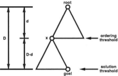
Because a process is interrupted and restarts when it receives new ordering information, each process search­ ing to a depth d will be interrupted by all processes searching to a shallower depth. This implies that the time to search to depth d is the sum of the times to search to each shallower depth. Since the tree grows ex­ ponentially, this has no effect on the asymptotic time complexity, which is still O(bd).

How long does it take to find a solution under these assumptions? The total time is the time for the ordering process to complete its search to depth d, plus the time for the solution process to complete the search below node x, which is of depth D-d. This is O(bd+bD-d). For small values of d, the running time is dominated by the time to perform the unordered search below depth d. For large values of d, the running time is dominated by the time to determine the ordering information. Note that ordering information doesn't help the ordering process, since the entire ordering threshold must be completed. The running time is minimized when d = D/2, which balances the two searches. This results in an overall complexity of O(bDf 2 ) in the best case.

In the above analysis, we defined D as the length of the first solution found. If we changed the definition of D to be the length of an optimal solution, then the same result applies to finding optimal solutions.

4.2.1 Number of Processes

Consider the minimum number of processes required to achieve this O(bDf 2 ) time complexity. All we need is enough processes so that the solution process can start as soon as the ordering process completes, or sooner. This is achieved with a minimum number of processes when the ordering process leapfrogs directly to become the solution process; this requires D/2 processes. Thus, D/2 processes are sufficient to find a solution in O(bDf 2 ) time. Note that having too few processes will delay the availability of a process for the solution threshold and thus increase the time to find a solution.

What is the effect of having more than the minimum number of required processes? Let D be the length of the optimal solution and consider what happens as we add more than D/2 processes. As discussed in section 3.2, if non-optimal solution density is greater than optimal solution density, we would find a non-optimal solution first and reduce the time to the first solution. On the other hand, if we add processes which search thresholds with relatively low non-optimal solution densities, then these processes will be unproductive since shallower so­ lutions will generally be found first. This implies that, depending on the problem domain, we may want to limit the number of windows for efficiency.

Even if the benefit of adding deeper windows de­ creases, however, parallel window search is not limited in how many processors it can effectively use. Once the desired window 'length' has been achieved, extra proces­ sors can be used to share in the search of each window. That is, more than one processor can search to a given threshold, for example usirig the approach of [Rao, 1987].

4.3 Empirical Results for First Solution Found

We ran the initial93 of 100 problems of [Korf, 1988] (or­ dered by nodes generated by serial IDA*) using a num­ ber of processors ranging from 5 to 9, and measured the time to find the first solution. The 7 most difficult prob­ lems weren't used because they would take too long to solve using 5 or 6 processors since this number is less than the minimum required as discussed in the previous section. All 100 problems, however were run using 7-9 processors with consistent results. In each case, we cal­ culated the average effective heuristic branching factor. The effective branching factor is one way of measuring the reduction in nodes generated. It tells how much the branching factor would have to be reduced in the serial search to find a solution in the time taken by the par­ allel search. Since the serial search requires O(bd) time and the parallel search in the best case requires O(bDf 2 ) = O(b·5D) = O((b·5)D), we expect an effective heuristic branching factor of at least b· 5 ·

4.3.1 Running Time Relative to IDA*

For 5, 6, 7, 8, and 9 processors, the corresponding average exponents of b were .8, .78, .75, .75, and .73, respectively. That is, we see a reduction of the heuristic branching factor to about b 3 1 4 · We believe b monotoni­ cally decreases for two reasons: (1) for the most difficult problems, adding extra processes helps achieve the min­ imum number of processes required (section 4.2.1); and (2) adding additional processes reduces the time to a so­ lution because of the density effect (section 3.2). The consistency of this reduction lends support to the claim that parallel window search reduces the exponential com­ plexity of IDA* for finding non-optimal solutions.

To give an idea of specific performance, when we ran all 100 problems using seven Hewlett Packard 9000/320 workstations, the average nodes generated in finding a solution was 1.6 million compared to an average of 357 million nodes generated in IDA*. More specifically, the most difficult problem IDA* solved required 42 hours and 6.01 billion node generations. Using 7 processors, our program found a solution to this problem that was 4 moves from optimal (6%) in 4 minutes and 6.5 million node generations (by the process finding the solution). If total processor effort is considered and not just elapsed real time, this corresponds to 28 minutes and 45 mil­ lion nodes generated; this is the time a single processor running PWS with 7 processes would take.

4.3.2 Solution Quality

The relative speed of the program is only one measure of its performance, with the quality of solutions being the other primary measure. For seven processors, the solution lengths range from optimal to twelve moves over optimal, with the mode and average being six moves over optimal. Since the average optimal solution length for this puzzle is 53 moves, the first solutions found are on the average within 11 percent of optimal.

To get a better indication of the strength of PWS in finding non-optimal solutions, we also compared it to RTA * [Korf, 1988), a real-time variant of A* in which optimality is sacrificed in order to make real-time moves within fixed time limits. In a sense, this is an unfair comparison since RTA * only searches from its current position in the sequence of moves made so far, but it is still instructive.

We compared the quality of solutions of PWS with 7 processors and RTA * as follows. RTA * was run with varying search horizons until it generated more nodes in finding a solution than all 7 processors of PWS. After removing any cycles from the solution, its length was compared to the PWS solution length. On the average the PWS solution lengths were half (47%) of the RTA* solution lengths. In only three cases was the RTA * solu­ tion shorter than the initial PWS solution, and in those cases it was 6 moves less in one case and 2 moves less in the other two cases. These results show that PWS is not dominated by either IDA* or RTA *, and thus it appears to be a competitive algorithm in terms of search effort versus solution quality.

5 Conclusions

The effectiveness of node ordering for improving the ef­ ficiency of IDA* is limited by the time to complete the previous iterations of the search. Conversely, window search in which different processes simultaneously perform different iterations, is limited by the time to com­ plete the final iteration. Combining effective node order­ ing with window search by sharing ordering information among processes makes it possible to find nearly optimal solutions quickly.

If the algorithm continues to run past the first solu­ tion found, it finds increasingly better solutions until an optimal solution is guaranteed or the available time is exhausted. Such behavior is important in real problems since: (1) a quick solution is often more important than an optimal one, and (2) problem solvers often have lim­ ited resources available to make a decision, and often cannot predict those resources apriori. In those situa­ tions, a problem solver must always have a plausible so­ lution available. Parallel Window Search provides such a capability.