Generalized Game Trees

1 Introduction

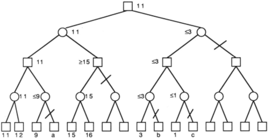
Minimax search with alpha-beta pruning is the pre­ dominant algorithm employed by two-player game programs[1]. Figure 1 shows a game tree, where squares represent Max nodes and circles correspond to Min nodes, along with its minimax value, bounds on interior nodes, and those branches pruned by alpha-beta.

There are two assumptions made in this model. One is that there are two players, and the other is that they both use the same evaluation function. Th.ere are, how­ ever, games that involve more than two players. Further­ more, the knowledge of different players is likely to be quite different in practice. First we will consider the con­ sequences for minimax and alpha-beta of assuming that two players use different evaluation functions. Next we will examine multi-player game trees. Finally, we will combine the two cases and briefly discuss multi-player games with different evaluation functions.

*This research was supported by an NSF Presidential Young Investigator Award, and NSF Grant IRI-8801939. Thanks to Chris Ferguson for helpful discussions concerning this work, and Valerie Aylett for drawing the figures.

2 Different Evaluation Functions

Given separate evaluation functions, there are two cases to consider, depending on whether or not each player knows his opponent's function.

2.1 Separate but Shared Knowledge

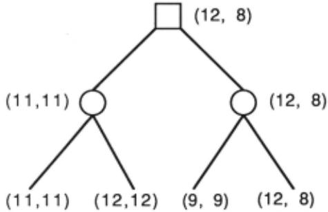
In the simplest case of separate evaluation functions, each player uses a different function and each player knows his opponent's function. This requires that min­ imax be modified as follows: Each node now has two evaluations, one for Max and one for Min. In figure 2, the first component is Max's value and the secon.d is Min's. The player to move at a given node uses h1s evaluation of the children, and backs up the complete ordered pair for which his component is a maximum or minimum, respectively.

In general, alpha beta pruning cannot be used in this case. Compare figure 2 with the two-level tree in the lower left corner of figure 1. Using either Max or Min's function exclusively would cause the last node to be pruned, yet its value is the minimax value of the root when both functions are used. The problem is that (12,8) is better than (9,9) for both Max and Min.

Pruning is possible only if the two evaluation func­ tions always agree on the relative ordering of the mer­ its of different positions. In other words, if one node looks better to Max than another, then it also must look worse to MIN. Since the actual values of positions don't matter, but merely their relative order, this constraint implies that both evaluation functions always make the same decisions, and hence are effectively identical. If two evaluation functions rank different positiobs differently, then alpha-beta pruning cannot be used and the entire tree must be searched.

2.2 No Shared Knowledge

So far we have assumed that each player knows his op­ ponent's function. Now we relax that constraint, and assume that each player merely has a model of his oppo­ nent's function, which may or may not be accurate. This is the most general and realistic case since in general one player can only guess at what his opponent may know. We will illustrate the necessary modification to minimax by a series of examples.

In a one-level game tree with Max at the root, Max simply applies his evaluation function to each of the chil­ dren, and chooses the one with the largest value.

In a two-level tree with Max at the root, Max's choice of move depends on what he thinks Min's move will be. Min's decision will be based on Min's evaluation of the terminal nodes, but Max only has a model of Min's func­ tion. Thus, Max applies his model of Min's evaluation to the frontier nodes, and backs up the position with the minimum value. Then, Max's evaluation function is ap­ plied to the two positions that are backed up, and the one with the maximum value is chosen for the move.

The situation gets more complex with a three-level tree. Again assume that Max is to move at the root. Max's decision will be based on what he thinks Min will do. However, Min's decision will be based on what he thinks Max will do two levels down. Thus, Max's deci­ sion is based on what Max thinks that Min thinks that Max will do. Therefore, the evaluation function that is applied to each of the frontier nodes is Max's model of Min's model of Max's evaluation, and the nodes with the maximum values are backed up to the Max nodes directly above the frontier. Next, Max's model of Min's evaluation is applied to the backed up nodes, and the nodes with the minimum values are backed up to the Min nodes directly below the root. Finally, Max's eval­ uation is applied to these backed up nodes to determine the final move.

In general, an additional level of knowledge is added for each level of the search tree. In theory, each of these different levels of knowledge could involve different eval­ uation functions. While the concept of multiple levels of knowledge is well-known in the game theory context of simultaneous decisions [2], alternating-move game trees provide a simple and often overlooked example of this phenomenon in artificial intelligence.

The restrictions on alpha-beta pruning in this case are the same as in the case of different but shared functions. In other words, the models of the different evaluation functions must agree in their relative ordering of different positions, which is to say that they must be functionally equivalent.

3 Multi-Player Game Trees

We now consider games with more than two players. For example, Chinese Checkers can involve up to six different players moving alternately. As another example, Othello can easily be extended to an arbitrary number of players by having different colored pieces for each player, and modifying the rules such that whenever a mixed row of opposing pieces is flanked on both sides by two pieces of the same player, then all the pieces are captured by the flanking player.

3.1 Maxn Algorithm

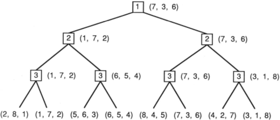
Luckhardt and Irani[3] extended m1mmax to multi­ player games, calling the resulting algorithm maxn. We assume that the players alternate moves, that each player tries to maximize his return, and is indifferent to the re­ turns of the remaining players. At the leaf nodes, an evaluation function is applied that returns an N-tuple of values, with each component corresponding to the esti­ mated merit of the position with respect to one of the players. Then, the value of each interior node where player i is to move is the entire N-tuple of the child for which the ith component is a maximum. Figure 3 shows a maxn tree for three players, with the corresponding maxn values.

For example, in Chinese Checkers, the value of each component of the evaluation function might be the neg­ ative of the minimum number of individual moves re­ quired to move all of the corresponding player's pieces to their goal positions. Similarly, an evaluation function for multi-player Othello might return the number of pieces for each player on the board at any given point.

The negamax formulation of two-player minimax is a special case of maxn for two players. The evaluation function returns an ordered pair of x and -x, and each player maximizes his component at his moves.

3.2 Alpha-Beta Pruning in Multi-Player Game Trees

Luckhardt and Irani[3] observed that at nodes where player i is to move, only the ith component of the chil­ dren need be evaluated. At best, this can produce a constant factor speedup, but it may be no less expensive to compute all components than to compute only one.

They correctly concluded that without further assump­ tions on the values of the components, pruning of entire branches is not possible with more than two players.

If, however, there is an upper bound on the sum of all components of a tuple, and there is a lower bound on the values of each component, then alpha-beta prun­ ing is possible. The first condition is a weaker form of the standard constant-sum assumption, which is in fact required for two-player alpha-beta pruning. The second is equivalent to assuming a lower bound of zero on each component, since any other lower bound can be shifted to zero by subtracting it from every component. Most practical evaluation functions will satisfy both these con­ ditions, since violating them implies that the value of an individual component can be unbounded in at least one direction. For example, in the evaluation function described above for multi-player Othello, no player can have less than zero pieces on the board, and the total number of pieces on the board is the same for all nodes at the same level in the game tree, since exactly one piece is added at each ·move.

3.2.1 Immediate Pruning

The simplest kind of pruning possible under these as­ sumptions occurs when player i is to move, and the ith component of one of his children equals the upper bound on the sum of all components. In that case, all remaining children can be pruned, since no child's ith component can exceed the upper bound on the sum. We will refer to this as immediate pruning.

3.2.2 Shallow Pruning

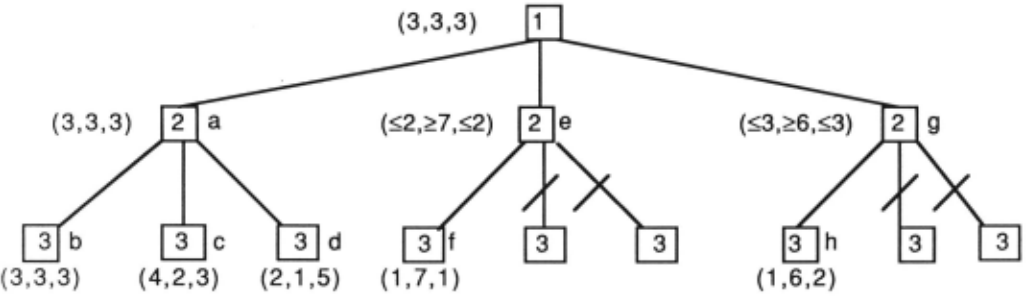
A more complex situation is called shallow pruning in the alpha-beta literature. Figure 4 shows an example of shallow pruning in a three-player game, where the sum of each component is 9. Evaluating node a results in a lower bound of 3 on the first component of the root, since player one is to move. This implies an upper bound on each of the remaining components of 9 - 3 = 6. Eval­ uating node f produces a lower bound of 7 on the sec­ ond component of node e, since player two is to move. Similarly, this implies an upper bound on the remaining components of 9 - 7 = 2. Since the upper bound (2) on the first component of node e is less than or equal to the lower bound on the first component of the root (3), player one won't choose node e and its remaining chil­ dren can be pruned. Similarly, evaluating node h causes its remaining brothers to be pruned. This is similar to the pruning in the left subtree of Figure 1.

The procedure Shallow takes a Node to be evaluated, the Player to move at that node, and an upper Bound on the component of the player to move, and returns a vec­ tor that is the maxn value of the node. Sum is the global upper bound on the sum of the components. Initially, Shallow is called with the root of the tree, the player to move, and Sum. Note that shallow pruning includes immediate pruning as a special case, and henceforth shal­ low pruning will be used to refer to both shallow and immediate pruning.

Shallov(Node, Player, Bound) IF Node is terminal, RETURN static value Best = Shallov(first Child, next Player, Sum)

FOR each remaining Child IF Best[Player] >= Bound, RETURN Best Next = Shallov(Child, next Player, Sum - Best[Player]) IF Next[Player] > Best[Player], Best=Next RETURN Best

3.2.3 Failure of Deep Pruning

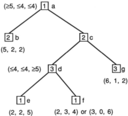
In a two-player game, alpha-beta pruning allows an additional type of pruning known as deep pruning. For example, In Figure 1, nodes b and c are pruned based on bounds inherited from their great-great-grandparent, the root in this case. Surprisingly, deep pruning does not generalize to more than two players.

Figure 5 illustrates the problem. Again, the sum of each component is 9. Evaluating node b produces a lower bound of 5 on the first component of node a and hence an upper bound of 9 - 5 = 4 on the remaining components. Evaluating node e results in a lower bound of 5 on the third component of node d and hence an upper bound of 9- 5 = 4 on the remaining components. Since the upper bound of 4 on the first component of node d is less than the lower bound of 5 on the first component of node a, the value of node f cannot become the value of node a. In a two-player game, this would allow us to prune node f.

With three players, however, the value of node f could effect the value of the root, depending on the value of node g. If the value of node f were (2,3,4) for example, the value of e would be propagated to d, the value of d would be propagated to c, and the value of b would be propagated to a, giving a value of (5,2,2). On the other hand, if the value of node f were (3,0,6) for example, then the value of f would be propagated to d, the value of g would be propagated to c, and the value of c would be propagated to a, producing a value of (6,1,2). Even though the value of node f cannot be the maxn value of the root, it can effect it. Hence, it cannot be pruned.

3.2.4 Optimality of Shallow Pruning

Given the failure of deep pruning in this example, is there a more restricted form of pruning that is valid, or is shallow pruning the best we can do? The answer is the latter, as expressed by the following theorem:

Theorem 1 Every directional algorithm that computes the maxn value of a game tree with more than two players must evaluate every terminal node evaluated by shallow prunmg.

By a directional algorithm we mean one in which the order of node evaluation is independent of the value of the nodes, and once a node is pruned it can never be re­ visited. For example, a strictly left-to-right order would be directional. The main Idea of the proof amounts to a generalization of the above example to variable values, arbitrary depth, and any number of players greater than two. Unfortunately, space constraints preclude us from including the proof here.

3.2.5 Best-Case Performance

How effective is shallow pruning in the best case? To simplify the analysis, we will exclude immediate pruning by assuming that no one component can equal the upper bound on the sum. The best-case analysis of shallow pruning is independent of the number of players and was done by Knuth and Moore[4] for two players.

In order to evaluate a node in the best case, one child must be evaluated, and then evaluating one grandchild of each remaining child will cause the remaining grand­ children to be pruned (see Figure 4). Thus, If F(d) is the number of leaf nodes generated to evaluate a tree of depth d with branching factor b in the best case, then F(d) = F(d- 1) + (b- 1) * F(d- 2). Since a tree of depth zero is a single node, and a tree of depth one re­ quires all children to be evaluated, the initial conditions are F(O) = 1 and F(1) =b. Note that in a binary tree, F(d) is the familiar Fibonacci sequence. The solution to the general recurrence has an asymptotic branching factor of (1 + vf4b- 3)/2. For large values of b, this ap­ proaches Vb which is the best-case performance of full two-player alpha-beta pruning.

3.2.6 Average-Case Performance

Knuth and Moore[4] also determined that in the aver­ age case, the asymptotic branching factor of two-player shallow pruning is approximately b /log b. They assumed independent, distinct leaf values.

In the case of multiple-players, however, our model of the evaluation function must have a lower bound on each component and an upper bound on their sum. For simplicity, assume that the lower bound is zero and that the sum is exactly one. Thus, we need a way of ran­ domly choosing N-tuples such that each component is identically distributed between zero and one, and the sum of all components is one. One way to do this is by cutting the zero-one interval in N - 1 places, with each cut-point independently and identically distributed from zero to one, and using the N resulting segments as the components of the N-tuple. Furthermore, we assume that each tuple is independently generated.

Under this average-case model, the asymptotic branching factor of shallow pruning with more than two players is simply b, the brute-force branching factor. The an~lysis relies on the minimax convergence theorem[1], which was derived for two-player minimax trees but also holds for multi-player maxn trees as well. This surpris­ ing phenomenon is that if the leaf values are chosen in­ dependently from the same distribution, the variance of the root values decreases with increasing height of the tree, and in the limit of infinite height, the root value can be predicted with probability one. The actual lim­ iting value depends on the leaf distribution and also on which player moves last in the tree, but the convergence does not.

In order for pruning to take place, the lower bound on one component must be greater than or equal to its upper bound, which equals one minus the lower bound on another component. Thus, pruning only takes place when the sum of the lower bounds on two different com­ ponents is greater than or equal to one. In order for this to occur in the limiting value, the values of the re­ maining components must be zero, since the sum of the two components in question is one. This cannot hap­ pen in the limiting value, assuming continuous terminal values. Thus, while pruning occurs at low levels of the tree, at higher levels it becomes increasingly rare, and in the limit of infinite depth, it disappears entirely. Thus, the asymptotic branching factor is simply b. This has been verified experimentally, using the model described above.

4 Multi-Player Games with Separate Evaluation Functions

What happens when we combine the assumptions of sep­ arate evaluation functions and multiple players? The re­ sult is a hierarchy of multiple functions, each of which returns a vector of values for each position. For example, in the three-player game tree of Figure 3, the evaluation function applied to the frontier nodes would be player 1 's model of player 2's model of player 3's evaluation function. At the next higher level, player 1 's model of player 2's function would be used, and finally player 1 's evaluation would be applied to the children of the root.

The constraints on alpha-beta pruning are the same. Namely, deep pruning cannot be done, and shallow prun­ ing can only be used where the corresponding functions behave identically. In the average case with more than two players, pruning does not reduce the asymptotic branching factor.

5 Conclusions

We have considered two extensions to the standard game-tree model. The first is to allow different play­ ers to have different evaluation functions, and different model's of their opponent's functions. In general, this produces a hierarchy of levels of knowledge that is as deep as the search tree to be evaluated. Furthermore alpha-beta pruning cannot be used unless the different evaluations are functionally equivalent.

The second is to allow an arbitrary number of play­ ers. This leads to a generalization of the minimax al­ gorithm called maxn. If we further assume that there is a lower bound on each component of the evaluation function, and an upper bound on the sum of all compo­ nents, then shallow alpha-beta pruning is possible, but not deep pruning. In the best case, this results in signif­ icant savings in computation, but in the average case it does not reduce the asymptotic branching factor.

This implies that alpha-beta is a rather specialized algorithm whose effectiveness is limited to the case of two-players with a common shared evaluation function. Since alpha-beta pruning is one of the main reasons for the effectiveness of the minimax backup rule, alternative backup rules may be more competitive in these more general settings.