
Experiences Implementing a Parallel ATMS on a Shared-Memory Multiprocessor
Proceedings of the Eleventh International Joint Conference on Artificial Intelligence. Parallel and Distributed Processing. Pages 199-204.
© 1989 International Joint Conferences on Artificial Intelligence
Abstract
The Assumption-Based Truth Maintenance System (ATMS) is an important tool in AI . So far its wider use has been limited due to the enormous computational resources which it requires. We investigate the possibility of speeding it up by using a modest number of processors in parallel. We begin with a highly efficient sequential version written in C and then extend this version to allow parallel execution on the Encore Multimax, a 16 node shared-memory multiprocessor. We describe our experiences in implementing this shared-memory parallel version of the ATMS, present detailed results of its execution, and discuss the factors which limit the available speedup.
- [deKleer, 1986] deKleer, J., "An Assumption-Based Truth Main- tenance System", Artificial Intelligence, 28, 1986.
- [Dixon and deKleer, 1988] Dixon, M. and deKleer, J. , "Massively Parallel Assumption-Based Truth Maintenance" , Proceedings of the National Conference on Artificial Inteligence, 1988.
- [Filman, 1988] Filman, R., "Reasoning With Worlds and Truth Maintenance in a Knowledge Based Programming Environ- ment", Communications of the ACM, 31, 1988.
- [Forbus, 1986] Forbus, K., "The Qualitative Process Engine", Uni- versity of lllinois Technical Report No. UIUCDCS-R-86- 1288, December, 1986.
- [Hillis, 1985] Hillis, D., The Connection Machine, MIT Press, Cambridge, Massachusetts, 1985.
- [Okuno, 1989] Okuno, H., "Parallel Execution of the ATMS on a Shared-Memory Multiprocessor", to appear.
- [Rothberg and Gupta, 1989] Rothberg, E. and Gupta, A., "Expe- riences Implementing a Parallel ATMS on a Shared-Memory Multiprocessor" , Stanford University Technical Report, May, 1989.
References were extracted automatically from the PDF and may contain errors.
Full text extracted automatically from the PDF; figures, tables and equations may differ. The PDF is the version of record.
1 Introduction
The Assumption-Based Truth Maintenance System (ATMS) is an important tool in AI. It makes the task of designing a problem solver much easier, removing the need for the problem solver to maintain information concerning derivations which it makes. With out an ATMS, the problem solver must implicitly record which of its assumptions it currently believes to be true and what these as sumptions imply. When it wishes to change its assumption set, it must also recompute the set of items which are implied. With an ATMS, the problem solver explores the problem space, informing the ATMS of the assumptions it makes, the items which it wishes to reason about, and the derivations which it makes concerning these items. The ATMS keeps track of which items hold under any given assumption set, thus allowing the problem solver to freely change the set of assumptions which it currently believes. A number of problem solvers have been built which use the ATMS in a num ber of AI subfields. The ATMS provides a convenient level of abstraction, greatly simplifying the structure of the problem solver [Filman, 1988].
So far wider use of the ATMS has been limited due to the enor mous computational resources which it requires. The ATMS is often the bottleneck in the problem solving process, often having greater computational requirements than the problem solver with which it is collaborating. We investigate the possibility of speeding up the ATMS by using a modest number of processors in paral lel. We begin with a highly efficient C-hased implementation of the ATMS based on the techniques described in [deKleer, 1986]. Through a number of modifications to the basic sequential ATMS, we obtain moderate speedup on the three example problem solver trace files which we examine.
*This research is supported by DARPA contract N00014-87-K0828. Edward Rothberg is also supported by an Office of Naval Research graduate fellowship. Anoop Gupta is also supported by a faculty award from Digital Equipment Corporation
The paper is organized as follows. Section 2 presents back ground information about the ATMS and introduces related termi nology. Section 3 presents details of an efficient sequential imple mentation of the ATMS. Section 4 presents the modifications to the sequential implementation which were necessary to allow parallel execution. Section 5 presents the results of executing the basic parallel implementation. We discuss the bottlenecks encountered and introduce a number of modifications to the basic algorithm to deal with these bottlenecks. Section 6 discusses related work, and Section 7 presents the conclusions.
2 The ATMS
The ATMS serves as a companion to a problem solver, acting as a sort of "truth database". The problem solver feeds beliefs, contradictions, and implications to the ATMS. The ATMS keeps track of what is true under what assumption sets and why. In this section we illustrate how the ATMS is used and introduce the terminology with a brief example. The example problem that we solve is the 3-queens problem, the problem of finding placements for three queens on a 3 by 3 chessboard such that no queen can capture any other.
Everything which the problem solver reasons about is assigned an ATMS node. In the 3-queens example we use 10 nodes, one for each of the 9 squares on the chessboard and one goal node to rep resent the solution. Each chessboard node represents the placement of a queen on the corresponding chessboard square. Some subset of the ATMS nodes are designated to be assumptions. These are nodes which are presumed to be true unless there is evidence to the contrary. In the example, the 9 nodes assigned to chessboard squares are the assumptions. We assume that a queen can be placed at each square of the board. Every important derivation made by the problem solver is recorded as a justification:
where Xt , xz, . .. are the antecedent nodes and n is the consequent node. In the example, the problem solver tells the ATMS that any set of three queens placed on the board constitutes a solution. Thus, the justifications take the form:
positiont , positionz , position3 =? goaLnode
where position; is an assumption which corresponds to a queen being on a particular square on the chessboard. An ATMS envi ronment is a set of assumptions. A node n holds in environment E if n can be derived from E using the current set of justifications. An environment is inconsistent (called nogood) if the distinguished node false holds in it. In the 3-queens example, we declare any set of assumptions in which the corresponding board positions contain a capturing pair to be nogood. The answer to the 3-queens prob lem is the set of all consistent environments in which the goal node holds.
In the ATMS, sets of envirorunents play an important role in keeping track of the contexts under which a given node holds. They are used extremely frequently, and consequently we need a concise representation for a them. In our representation, we can take advantage of the fact that if a node holds under envirorunent E, then it also holds under any superset of E. Also, any node holds under a nogood environment, so it is never necessary to keep track of nogoods in the set. We therefore represent a set S of envirorunents by its smallest consistent members, a list of envirorunents (£1 , E2 , .. . ), which we call a minimal environment list. This representation has the following properties:
- Minirnality - No E; is a subset of any other.
- Consistency - No E i is nogood.
The distinction between sets of environments and sets of assump tions presents a possible source of confusion. For example, con sider the envirorunents {A, B} and {A, B, C}. Clearly {A, B, C} is a superset of {A, B}. Yet, the minimal envirorunent list ( {A, B, C}) represents a subset of the minimal environment list ( {A, B} ); the second contains envirorunents which do not have assumption C in them, while the first does not. Please keep this potential source of confusion in mind when we discuss envirorunent supersets and subsets in the remainder of this paper.
The problem solving process involves a dialogue between the problem solver and the ATMS, in which the ATMS receives a se quence of requests to create new nodes, new assumptions, new justifications, and to provide information on the envirorunents in which nodes hold. This information can be easily provided if the ATMS maintains with each node n a set of envirorunents, in mini mal envirorunent list form, called its label. In addition to its mini mal envirorunent list properties, each node's label has the following two properties:
- Label soundness - Node n holds in every envirorunent in the label set.
- Label completeness - Every envirorunent E in which n holds is a member of the label.
3 Sequential Implementation
We now examine how the sequential ATMS is actually imple mented, with emphasis on those aspects of the implementation which are relevant to parallel execution. Since we will be com puting the speedups of the parallel implementation based on the execution time of the sequential implementation, we must make sure that sequential version is as efficient as possible.
3.1 The Trace Files
We first present the results of executing three problem solver traces on our ATMS. These traces were generated by monitoring the in teraction between an actual problem solver and an ATMS, and dumping the observed interaction into a trace file. The traces are:
- QPE, from a problem solver created by Ken Forbus [Forbus, 1986] which solves Qualitative Physics problems.
- BUG, a trace which led to a bug in some ATMS implemen tation.
- 8-Q, from a problem solver which solves _the 8-queens prob lem. This formulation of theN-Queens problem differs some what from the one described earlier in this paper.
Table 1 provides information on the three traces. It also provides the runtimes for the three traces, both for the LISP-based ATMS implementation of deKleer [deKleer, 1986] and for our C-based implementation. We provide these numbers to demonstrate that we are basing our parallel program on an efficient sequential imple mentation. The time quoted for deKleer's ATMS is from execution on a Texas Instruments Explorer I lisp machine. The time quoted for our implementation is from execution on a single processor of an Encore Multimax multiprocessor. The Encore MultiMax is a 16 node, shared-memory multiprocessor, with an NS 32032 (0.75 MIPS) microprocessor at each node. We also include the runtime on a more widely available machine, a DEC DecStation 3100, for reference purposes. These times include all costs involved in pro cessing the trace files from beginning to end, including the time spent processing the ATMS commands and the time spent reading the trace files from disk.
| QPE | BUG | 8-Q | |
|---|---|---|---|
| Nodes | 988 | 1705 | 131 |
| Assumptions | 38 | 62 | 64 |
| Justifications | 2584 | 4165 | 1192 |
| Run time (in seconds) | |||
| - deKleer's on Explorer I | 125 | 221 | ? |
| - ours on MultiMax | 38.9 | 89.7 | 35.1 |
| - ours on DecStation 3100 | 2.2 | 4.8 | 1.9 |
3.2 Implementation Overview
The four basic operations which the ATMS makes available to the problem solver are:
- Create-Node n - create a new node.
- Create-Assumption n - -create a new assumption.
- Justify-Node n by x 1 x2 ... - add a new justification.
- Node-Query n - request the current label of node n.
The problem solver places a sequence of these commands on a queue it shares with the ATMS. The ATMS repeatedly removes available commands from this queue. Given a command, it per forms the requested action, restores node label soundness and con sistency for all nodes in the inference graph, and is then ready to perform the next command.
Of the four commands which the ATMS makes available to the problem solver, only Justify-Node consumes significant amounts of time. The Create-Node command takes very little time, since at the point at which the node is created it does not participate in any jus tifications. The Create-Assumption command also takes little time for the same reason. The Node-Query command is also computa tionally inexpensive because of the properties of label consistency, soundness, completeness, and minimality. In order to process a Node-Query command, the ATMS simply returns the current label of the appropriate node.
When a Justify-Node command arrives at the ATMS, the labels of the consequent node n and any nodes which depend on node n may no longer be complete. Node n may now be derivable from a new set of assumptions not currently in node n 's label. Its label must be updated, and any changes to node n' s label must be propagated to the successors of node n.
A new justification can also cause new nogood environments to be discovered, potentially causing the node label of any node in the inference graph to become inconsistent. The simplest example of this would be a justification whose consequent is the false node. In order to restore node consistency, environments which become nogood must be removed from all node labels.
In order to handle propagation of node labels, the ATMS main tains an Update request stack. Any time a node label is changed, Update requests are placed on the request stack, one for each jus tification which has the modified node as an antecedent. The first step in the processing of a new justification is to push an Update request onto the request stack. The ATMS continues popping Up date requests off of the Update stack, processing the requests, and potentially pushing more requests onto the stack until the stack is empty. This corresponds to a depth first propagation of labels.
A single Update request is processed as follows:
- The set of consistent environments which derive the conse quent using the new justification and the new label environ ments is computed. This set is the intersection of the new label environments of the one antecedent with the labels of the other antecedents of the justification.
- If the consequent is the false node, then all of these environ ments are recorded as nogood.
- Otherwise, the consequent node label is set equal to the union of the previous label and the new set of environments.
- The changes to the consequent label, i.e. the set of environ ments in the label which were not present in the previous label, are propagated to all nodes which depend on the con sequent.
3.3 Set Operations on Minimal Environment Lists
Adding a new justification requires a number of set operations on sets of environments, including set union and set intersection. The minimal environment list representation allows us to perform these operations quickly. Given two environment sets, S and T, rep resented as (£1, £2 , ... ) and (F1 , F2 , . .. ) respectively, we perform set operation on them as follows:
When we wish to add a new set of environments to the label of a node, we must take the set union of the existing label with the set of new environments. The set union of S and T, in minimal form is the concatenation of the minimal forms of S and T, with all supersets removed.
When we wish to compute the effect of a justification on its consequent node, we must find the set intersection of all of the labels of the antecedent nodes. The set intersection of S and T is somewhat more involved than the set union. If all supersets of E; are in S and all supersets of F1 are in T, then all environments which are supersets of both E; and F 1 are in S n T. The set of all supersets of both E; and F1 is the set of all supersets of the union of £; and F 1 (remember that environments are sets of assumptions). For example, the intersection of the supersets of {A. B} with the supersets of { B , C} is the supersets of {A, B, C}, which is the union of {A , B} with { B, C}. Thus the intersection of S with T is the set of all supersets of the pairwise unions of E; with F1 · Thus, in minimal environment list form, this is the cross product of the minimal environment list forms of S and T, again with all supersets removed.
3.4 Data Structures
The efficiency of the ATMS is highly dependent on the data struc tures and algorithms used in the implementation. A straightforward ATMS implementation can literally take days to solve a problem which a more sophisticated implementation solves in a few min utes. We first present the major data structures used in our ATMS implementation. The data structures are simply laid out here with brief descriptions; the purpose of each individual field will be made clear in later sections.
The environment data structure has the following fields: (1) Present: a bit vector representing the set of assumptions present in the environment. (2) Constituents: a list of all assumptions present in the environment. (3) Size: the number of assumptions present. (4) Contra: a flag indicating whether the environment is consistent. (5) Where: a list of all nodes which contain this environment in their labels. (6) Orthogonal: a bit vector representing the set of assumptions which, if added to the environment, would result in a nogood environment.
The node data structure has the following fields: (1) Label: the node's label. (2) Assumption: a pointer to the node's assumption fields, if the node is an assumption. (3) Consequences: a list of justifications in which the node is an antecedent.
The assumption data structure has the following fields, in addi tion to its node fields: (1) Binary: a bit vector representing the set of all binary nogoods this assumption participates in. If bit j is set in the Binary field of assumption i, then the environment {i, j} is nogood. (2) Nogoods: a table of all minimal nogood environments in which the assumption belongs, indexed by environment size.
The justification data structure has the following fields: (1) An tecedents: a list of antecedent nodes. (2) Consequent: the conse quent node.
3.5 The Environment Database
Our ATMS maintains three data structures to keep track of envi ronments encountered during a problem solver run, an environment hash table, a Consistent table, and a Minimal Nogood (MNG) table. The environment hash table holds all environments encountered so far, both consistent and nogood, indexed by a hash function. The Consistent table holds all consistent environments, and is indexed by environment size (number of assumptions present in the envi ronment). The MNG table holds all minimal nogoods, the nogoods which are not subsumed by any other nogood, and is again indexed by environment size. Each environment has a unique physical rep resentation in memory.
We make two modifications to the simple MNG table for ef ficiency. First, we handle unary and binary nogoods as special cases. The assumption data structure has a field entitled Binary which keeps track of unary and binary nogoods. If bit j in the Binary field of assumption i is set, then the environment { i , J} is nogood. Similarly, if bit i is set, then { i} is nogood. The second modification involves the Nogood field of the assumption data structure. Any environment in the MNG table is also kept in the Nogoods table of each assumption in the environment. These two modifications allow the ATMS to find all minimal nogoods containing a given assumption extremely quickly.
The Consistent and MNG tables form what we call the envi ronment database. The environment database, together with the environment hash table, make the following frequent operations extremely fast:
- When searching for a particular environment, find its unique representation.
- When checking an environment for consistency, find all min imal nogoods smaller than that environment.
- When adding a new nogood, find all consistent and nogood environments larger than that environment.
We represent an environment as a bit vector. A one in bit i of the vector indicates the presence of assumption i in the environ ment. This representation allows us to do subset testing, the most prevalent operation in the ATMS, by simply ANDing the bit vector of one environment with the complement of the bit vector of the other environment. The bit vector representation also allows fast hash function computation.
3.6 The Cross Product
When we handle an Update request, we need to compute the cross product of a number of mirrimal environment lists, as was described previously. Assume we wish to take the cross product of n min imal environment lists h, h, ... , ln, with l1 being the incremental update. We do this by looping over each list, creating m ,, the cross product of 11 through/;. We begin with m1 = /1, and at each iteration we compute m,+l = m; x li+l. where both m, and ffii+l are in minimal environment list form. We do this by collecting the unions of each environment E in m ; with each environment F in li+l, again with supersets removed.
We can greatly decrease the amount of time it takes to compute m 11 by using the following two techniques. First, if some envi ronment E in m; is subsumed by some environment in the label of the consequent of the justification which we are updating, then clearly every environment in m;+1 ... mn which is generated from E will also be subsumed by this environment. Any such E may therefore be discarded.
Second, consider taking the cross product of m ; with l;+ I· If some environment E in m ; is subsumed by some F in l ; + 1 , then clearly E will be in m;+l· Since all environments which would result from taking the union of E with some environment in l; + 1 are supersets of E and since E is in m i+ 1, none of the resulting environments will be present in m;+l· We can therefore place any such E into m;+1, thus avoiding having to take the union of E with each environment in m, +I ·
If we compute the cross product, using these two techniques, the result is a minimal environment list which represents the change to the label of the consequent node n. If the consequent is not the false node, we add each environment in our cross product to the label of node n. We must now restore minimality in the label by checking every environment previously in the label for subsumption against every environment just added to the label. We then propagate the cross product list, which represents the changes to the label of node n, to every justification which has node n as an antecedent.
If the consequent is the false node, then our cross product list is a set of environments which were previously consistent but have just become nogood. We add them to the MNG table, and sweep through the Consistent and MNG tables looking for subsumed en vironments. If an environment in the Consistent table is subsumed, it is removed from the table and from the labels of all nodes which contain it (found in the Where field of the environment). If an environment in the MNG table is subsumed, it is removed from the table.
Computing the union of two environments is an extremely fre quent and potentially extremely costly operation in the ATMS. The method of union computation which we use is an assumption by assumption method. That is, given two environments E 1 and E2, we compute the union by successively adding the assumptions in E2 into E1, computing an intermediate environment at every step. The result of a union is either a consistent environment E 3, which is the union of E1 with E2, or nogood, indicating that the union of E1 with E2 is nogood. While this seems like a somewhat cum bersome way of computing the union, if we look at the amount of worlc done per union we see that in practice it is extremely effec tive. In QPE, BUG, and 8-Q, the average number of assumptions which must be added to E1 before the union is known are 1.05, 1.04, and 1.00, respectively.
While the exact details of the union computation are crucial to the efficiency of a sequential implementation, they are not essential to understanding the parallel modifications which follow. Briefly, the Orthogonal field of the environment and the Binary field of the assumption (see Section 3.4) allow the ATMS to quickly determine when adding an assumption to a particular environment will result in a nogood. If these quick tests fail, then the environment must be checked for its existence in the hash table, and if it doesn't exist it must be checked for consistency with the minimal nogoods.
This concludes our discussion of an efficient sequential imple mentation of the ATMS. As was discussed in section 3.1, our im plementation is quite competitive with existing ATMS implemen tations. We use the sequential implementation which we have de scribed as the basis of comparison for the parallel implementations which we describe in the remainder of this paper.
4 Modifications for Parallel Implementation
We now discuss the modifications which are necessary to allow the preceding algorithm to be executed in parallel on a modest number of processors. Our goal is to exploit as much parallelism as possible, but we can not afford to introduce a large amount of redundant worlc in doing so.
4.1 Division of Work
The overall structure of our parallel ATMS is quite similar to the structure of the sequential ATMS. The ATMS and the problem solver run concurrently, sharing commands and data through a shared command queue. In order to allow a greater amount of par allelism, we no longer require that node labels be made sound and complete at the completion of each command. This requirement would necessitate the synchronization of all processors after each command, an operation which would greatly constrain our ability to distribute worlc among the processors. We now only require that labels be made sound and complete before a Node-Query command is answered. Thus, Node-Query commands are now somewhat ex pensive, since they require a global synchronization. Create-Node and Assume-Node messages again require very little work to be done, and are dealt with quickly. Justify-Node agalli require by far the most computation time, and thus afford the most opportunity to distribute worlc.
In order to decrease contention for tasks, each processor has its own Update request stack. When a processor completes a task, it first looks for a new task in it's own Update request stack. If it is empty, then the processor checks the global command queue. If the next command on the command queue is a Node-Query (or if the command queue is empty) the processor becomes idle. When all processors are idle, one processor processes and removes the Node Query command, thus unblocking the problem solver and allowing the problem solving process to proceed. We call this Program Pl. We later provide variations of this basic algorithm.
4.2 Locks
In our shared memory implementation, all the processors access the same data structures. We therefore need a number of mutual exclusion locks to control simultaneous access to shared data We begin by using straightforward locking techniques, and later modify our approach based on the observed bottlenecks.
Our ATMS implementation has a number of local structures, where access and modifications to these structures has little or no effect on other structures. These include the environment hash table buckets, the environments, and the ATMS nodes. We provide a lock for each one of these structures to enforce the following conditions: For hash table buckets, no two processors may access the same bucket at the same time. For environments, we enforce the conditions that no nogood environment may be added to a node's label and when an environment becomes nogood, it must be removed from the label of every node which contains it, and that only a single processor may change an environment from good to nogood. For nodes, we enforce the condition that no node label may be accessed by more than one processor at the same time. In order to decrease contention when processing justification updates, we copy the node label and worlc with the copy. Since a typical ATMS application has thousands of each of these structures and for now we are using at most 16 processors, contention for these locks is usually not a problem.
In contrast to the relatively local structures which we have just discussed, the environment database is a very global structure. A single change could conceivably affect every environment in the environment database. We must be able to check a new environ ment for consistency against all nogoods encountered so far. We must also allow a new nogood to be added and all existing environ ments to be checked for consistency against this new nogood. Since the ATMS spends much of its time creating new environments and checking them for consistency, we cannot tolerate a high latency on consistency checking. At the same time, however, most new environments which are encountered are nogood, so to avoid su perfluous worlc we want a new nogood to be recorded as soon as possible. We initially used a single global lock to control access to both the Consistent and MNG tables. Since the ATMS spends a substantial percentage of its time within this lock (3-15% for the three traces), this global locking approach appears somewhat suspect.
| QPE | BUG | 8-Q | ||||
|---|---|---|---|---|---|---|
| P1 | P2 | P1 | P2 | P1 | P2 | |
| Tasks | 2584 | 18780 | 4165 | 16576 | 1192 | 3308 |
| Avg task time (s) | O.oi5 | 0.002 | 0.019 | 0.005 | 0.028 | 0.010 |
| Max task time (s) | 2.42 | 0.86 | 35.31 | 6.88 | 0.36 | 0.34 |
| Total runtime (s) | 39.34 | 39.34 | 82.31 | 82.31 | 33.72 | 33.72 |
5 Results
We now present the results of executing the three problem solver traces on our parallel ATMS. Note that because Node-Query in formation was not required when the traces were originally gener ated, these traces do not record this command. The absence of this command does not affect the performance of the sequential ATMS significantly, since Node-Query commands take so little time to ex ecute. In our parallel ATMS, however, the lack of these commands obviates the need for global synchronization. Thus, the results we present here are optimistic, as the synchronization is done only at the completion of the entire trace. In applications where Node Query commands are frequent, one would expect less available parallelism.
The ATMS traces we examine seem to present abundant oppor tunities for parallelism. Their inference graphs are extremely large, with thousands of justifications capable of being distributed among the processors (see Table 1). Though the only limiting factor would appear to be the global lock on the Consistent and MNG tables, we observed speedups of only 3.9, 1.6, and 6.5 for QPE, BUG, and 8-Q, respectively, when Program 1 was executed on 14 processors. These were greatly below what one would expect, even given the global lock. The sequential ATMS spends 3%, 15%, and 6% of its time within the lock for the three traces. H this were the only parallelism limitation, we would expect speedups of 7 or more. Clearly, parallelism is being limited in some other way.
The most serious bottleneck appears to be processor idle time. When executed on 14 processors, the processors spend 54%, 72%, and 5% of the total runtime, for QPE, BUG, and 8-Q, respectively, without a task to execute. We have a number of tasks of varying size to execute, and we wish to divide them among a number of processors so that each processor takes approximately the same amount of time to complete them. This near equal division of tasks is usually possible given a large number of tasks to distribute; the large number of tasks serve to smooth out the variations in grain size. However, two factors make this untrue in Program Pl. First, the variation in grain size is enormous. In the BUG trace, for example, the processing of a single justification accounts for 43% of the run-time of the trace (see Table 2). Second, as the trace progresses the size and complexity of the inference graph increases, thus making the amount of work involved in processing a justification increase. The combination of some extremely large grains with the tendency for the large grains to be towards the end of the trace combine to make it extremely likely that one processor will be stuck with a large grain while the other processors have nothing to worlc on.
In order to alleviate the grain size problem, we decrease the task size. Instead of each problem solver issued command being a single task, we now consider each Update request to be a task. In Program P1, once the command queue becomes empty the proces sor simply quits. Now, in Program P2, an idle processor attempts to steal an Update request from the Update stacks of the other processors. In this way, work can be distributed among the proces sors even after the command queue has been emptied. Comparing columns in Table 2 we see that by decreasing the task size we have greatly increased the number of tasks and greatly reduced both the average and maximum task size. The net result of our modilica tion (Figure 1) is that the speedup is greatly increased from that of Program P1, but it is still far from ideal.
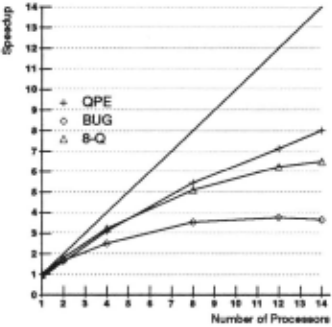
Another serious bottleneck in our parallel implementation is the environment database lock. In order to increase concurrency in the environment database, we introduce another variation on our basic algorithm. In Programs P1 and P2, only a single processor may access the database at one time. Our modilication, which we call Modal access, allows a number of processors to access the table concurrently, while still maintaining the stringent consistency requirements of the environment database.
The problem in allowing concurrent access to the database comes from the potential simultaneous additions of a consistent environment and a nogood environment. In order to add the con sistent environment to the database, we must know that it is not subsumed by any environment in the MNG table. To add the no good to the database, we must remove all environments which are subsumed by it from the Consistent table. These requirements seem to place serious sequentiality constraints on modilications to the en vironment database. In order to avoid these constraints, we add a mode of access indicator. The three access modes are Free mode, in which no processor is currently accessing the database; Consis tent mode, in which only consistent environments may be added to the database; and NG mode, in which only nogood environments may be added to the database. H a processor wishes to add a new consistent or nogood environment and finds the database in the wrong mode, it must wait until the conflicting access is complete.
We can modify the above slightly to increase concurrency. When new nogood environments are generated, they usually come in groups of more than one. We can therefore distribute the worlc of adding a list of new nogoods among a number of processors. New nogoods waiting to be added are placed on a global list. Now when a processors wishes to add a consistent environment and finds the database in NG mode, instead of waiting for the mode to change, the processor pulls new nogood environments off of the global list and processes them.
Figures 3 and 4 show the percentage of time each processor spends doing useful worlc as compared to the percentage spent waiting on locks and the percentage spent idle for two of the three traces executed with Program P3. The numbers for the third trace are between those of the two presented. The speedups obtained from Program P3 (Figure 2) are still far from ideal. While con tention for the environment database is greatly reduced, it is still substantial. We also still have a substantial speedup reduction due to processor idle time.
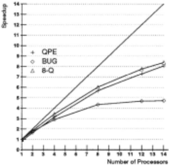
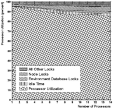
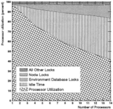
Note that the speedup obtained is not equal the product of the processor utilization and the number of processors used. This is due to several factors. First, our speedup numbers are obtained by dividing the parallel execution time by the execution time of the best sequential implementation. There are a number of over heads involved in the parallel implementation, such as environment list copying and redundant checks, which can reduce the speedup when compared to a sequential implementation without these over heads. Second, the parallel ATMS does not necessarily do the same amount of work that the sequential ATMS does. For example, the parallel ATMS can process the justifications in a different order than the sequential ATMS. While the answer we arrive at is the same, the amount of propagation necessary to get to this answer may differ. Third, there a number of hardware contention issues, including bus bandwidth and cache interactions, which can preclude linear speedups. We noticed a substantial degradation in speedup (as much as 30%) which could not be attributed to software issues and must therefore be caused by hardware contention. These issues are not reflected in the utilization graphs which we present.
We have yet to examine one possible cause of reduced speedup in the parallel implementation, redundant work. In the ATMS, it is difficult to establish a measure of how much "work" is being done. There are a number of routines which are called often and take large amounts of time, yet none dominates the others. One routine, subset testing, accounts for more of the runtime of the se quential ATMS than any other routine, and appears in many diverse places in the computation. It therefore appears to be a reasonably accurate measure of work. According to our subset measure of work, we observed that the parallel ATMS does between 90% and 106% of the work of the sequential ATMS for 14 or fewer pro cessors. Though the subset test numbers show interesting trends as the number of processors grows larger, the differences for less than 14 processors are not significant.
5.1 Going to a Still Finer Grain
Variation in grain size is still a problem in our implementation. Fur thermore, the problem would be much more severe if Node-Query commands were more frequent. One possible way to further de crease the grain size would be to split Update requesis into smaller pieces. In Program P3, an Update request contains a list of new environments which have been added to the label of an antecedent. In order to decrease the size of a single grain, we could split this list into many smaller lists. We could use a heuristic to determine approximating how long an Update task will take. Depending on the estimate, the list can be split so that other processors will not go idle while this task is executed. In the extreme, Update requests can be split into single new antecedent environments.
Performing Updates with smaller lists of environments can gen erate a large amount of avoidable work, however. Consider the cross product of ( {A} . { B} , { C} , { D} ) with ( { D} ) If we sim ply perform the cross product, we get the list ( { D} ). If we split the list ( {A} , { B} , { C} , { D} ) into two parts and perform separate cross products, however, we get ( {A, D} , { B , D} ) from the first part and ( { D} ) from the second. Now, instead of propagating a single list of length one to the successors of the consequent, a list of length two and a list of length one are propagated.
We can observe this situation in the BUG trace file. The largest Update task in the trace arises from a justification x 1 , x 2 , X3. X4 , X5 => n. The Update request comes from x 1 with a list of 8 new environments. Nodes x 2, X3, and X4 all have 8 envi ronments in their labels, and node x 5 has 1 environment in its label. The resulting cross product environment list contains 293 environ ments, If the incoming new environment list of 8 environments is split into two environment lists of 4 environments each, one result ing cross product contains 367 environments and the other contains
55. The net effect of splitting this single Update request into two smaller requests is substantial. The sequential execution time for BUG increases from around 82.31 seconds to 119.96 seconds, an increase of 46%. While we could have all processors working on a single Update synchronize and combine their results before propa gating them on, the added synchronization combined with the fact that the pieces of a split Update are not necessarily smaller than the whole Update combine to make such an action unwise.
Due to the above reasons, our initial efforts to go to a smaller grain have not resulted in much success. In order to get signifi cantly more speedup from some ATMS instances, we need to :find a natural task grain which is smaller than that of an Update request. Unfortunately, no obvious alternative presents itself.
6 Related work
While in this paper we have explored how ATMS parallelism can be exploited on a shared-memory multiprocessor, a related question is how it can be exploited on other types of parallel machine archi tectures. Mike Dixon and Johan de Kleer have proposed [Dixon and deKleer, 1988] a Massively Parallel Assumption-Based Truth Maintenance System, which we refer to as the MPATMS. This MPATMS can utilize thousands of processors, thus potentialy mak ing possible the extremely fast solution of large ATMS problems. For example, on the N-Queens problem they achieve speedups of around 100 running on a 16K processor Connection Machine [Hillis, 1985] over a sequential ATMS running on a Symbolics Lisp Machine.
As Dixon and deKleer discuss in the paper, their MPATMS has a strong relation to chronological backtracking. Specifically, the number of processors which execute a specific command in the MPATMS is exactly equal to the number of times the command is executed by a sequential backtracker. In other words, the MPATMS preforms the same amount of work as a sequential chronological backtracker, though, of course, the work is done in parallel. The problem, however, is that chronological backgracking is not the most efficient form of backtracking. More efficient techniques such as dependency directed backtracking exist. In fact, the ATMS was designed by deKleer as a means of dealing with the limitations inherent in backtracking. The ATMS avoids the main source of inefficiency in backtracking, the rederivation of previously derived conclusions. As an example of this efficiency, Ken Forbus [Forbus, 1986] has developed a pair of problem solvers in the domain of qualitative physics. He finds that QPE, his ATMS based problem solver, is approximately 95 times faster than his backtracking based GIZMO.
In the above context, while a 100-fold speedup for theN-Queens problem appears promising, several factors must be considered. First, the Symbolics LISP machine is a relatively slow machine. More modem machines offer many times the performance. Second, the N-Queens problem is one for which the ATMS offers no advan tage over chronological backtracking. A backtracker will perform no redundant derivations when solving this problem. On problems which are less amenable to solution by chronological backtracking, we would expect substantially less speedup. Thus, it remains to be seen whether this approach will offer significant speedups for ATMS problems from a wide range of domains.
Work is also being done by Hiroshi Okuno on a parallel QLISP based ATMS [Okuno, 1989].
7 Conclusions
In this paper, we have presented the details of implementing both a sequential and a parallel ATMS. The results we obtained from ex ecuting the parallel implementation on an Encore MultiMax allow us to draw a number of conclusions.
- The traces we examined seemed to present abundant op portunities for parallelism. They consisted of thousands
of relatively independent tasks, seemingly capable of being distributed among a number of processors. However, this apparent abundance of parallelism proved to be somewhat elusive to exploit.
- The obvious source of parallelism in the ATMS, the thousands of justifications, generated grains which varied enormously in size. In one trace, for example, a single justification ac counted for 43% of the total runtime, making effective paral lel distribution of grains impossible. In order to make grain sizes more uniform, we decreased the grain size by treating a single justification update as a task. We also introduced the notion of modal access to the environment database in order to alleviate the sequentiality constraints imposed by the global consistency requirements.
- With these modifications, we were able to obtain speedups of between 4.7 and 8.4 using 14 processors for the three trace files which we examined. Further speedups were limited by a number of factors, including still too large a variation in task grain size, processor contention for numerous mutual exclusion locks, and hardware contention issues.
- Although the parallelism is limited, by combining it with a highly efficient C-hased implementation we have created an ATMS implementation which is significantly faster than cur rently available LISP-based implementations.
- Finally, despite significant efforts made by us, any attempts at increasing the available parallelism in the ATMS by reducing grain size resulted in an explosion in the amount of work done. This explosion of work is also present in the massively parallel approach to the ATMS. Consequently, a major new insight is needed if we are to obtain significant speedup from parallel processing.
A more detailed version of this paper can be found in [Rothberg and Gupta, 1989].
Acknowledgments
We would like to thank Johan deKleer and Ken Forbus for pro viding us with ATMS trace files . We would like to thank Hiroshi Okuno for his assistance in the initial stages of this research.
@inproceedings{ijcai1989p32,
  title     = {Experiences Implementing a Parallel ATMS on a Shared-Memory Multiprocessor},
  author    = {Rothberg, Edward and Gupta, Anoop},
  booktitle = {Proceedings of the Eleventh International Joint Conference on
               Artificial Intelligence, {IJCAI-89}},
  publisher = {International Joint Conferences on Artificial Intelligence},
  editor    = {N. S. Sridharan},
  pages     = {199--204},
  year      = {1989},
  month     = {8},
  note      = {Parallel and Distributed Processing},
  url       = {https://ijcai.org/proceedings/1989/32},
}
TY - CPAPER TI - Experiences Implementing a Parallel ATMS on a Shared-Memory Multiprocessor AU - Rothberg, Edward AU - Gupta, Anoop T2 - Proceedings of the Eleventh International Joint Conference on Artificial Intelligence, IJCAI-89 PB - International Joint Conferences on Artificial Intelligence PY - 1989 SP - 199 EP - 204 UR - https://ijcai.org/proceedings/1989/32 ER -Copied
Machine-readable versions of this paper, for tools and AI agents:





