
Unsupervised Learning by Backward Inhibition
Proceedings of the Eleventh International Joint Conference on Artificial Intelligence. Parallel and Distributed Processing. Pages 170-174.
© 1989 International Joint Conferences on Artificial Intelligence
Abstract
Backward inhibition in a two-layer connectionist network can be used as an alternative to, or an enhancement of, the competitive model for unsupervised learning. Two feature discovery algorithms based on backward inhibition are presented. It is shown that they are superior to the competitive feature discovery algorithm in feature independence and controllable grain. Moreover, the representation in the feature layer is distributed, and a certain "classification hierarchy" is defined by the features discovered.
- [Ackley et al., 1985] D.H. Ackley, G.E. Hinton, and T .J. Sejnowski. A learning algorithm for Boltzmann machines. Cognitive Science 9:147-169, 1985 .
- [Anderson, 1986] J.A. Anderson. Cognitive capabilities of a parallel system. In E. Bienenstock et al. (Eds.), Disordered Systems and Biological Organization. Springer-Verlag, Berlin, 1986.
- [Ballard, 1987] Ballard, D.H .. Modular learning in neural networks. In Proceedings of the National Conference on Artificial Intelligence, pages 279-284, Seattle, 1987.
- [Chun et al., 1987] H.W. Chun, L.A. Bookman, and N. Afshartous. Network regions : alternative to the winner-take-all structure. In Proceedings of the Tenth International Conference on Artificial Intelligence, pages 380-387, Milano, 1987.
- [Dalenoort, 1987] G.J. Dalenoort. Development of concepts . Cognitive Systems 2(1) :123-140, 1987 .
- Fukushima, 1980)
- K. Fukushima . Neocognitron: A self-organizing neural network model for a mechanism of pattern recognition unaffected by shift in position . Biological Cybernetics 36:193-202, 1980.
- Grossberg, 1982)
- S. Grossberg. Studies of Mind and Brain. D. Reidel Publishing Co .. Dordrecht, 1982
- [Grossberg, 1987] S. Grossberg. Competitive learning: From interactive activation to adaptive resonance. Cognitive Science 11:23-63, 1987.
- Hinton and Lang, 1985) G.E . Hinton and K.J. Lang. Shape recognition and illusory conjunctions. In Proceedings of the Ninth International Conference on Artificial Intelligence, pages 252-259, Los Angeles, 1985. IJCAI
- Hinton et al., 1986) G.E. Hinton, J .L. McClelland and D .E. Rumelhart . Distributed Representations. In D .E . Rumelhart and J.L. McClelland (Eds.), Parallel Distributed Processing, Volume 1. MIT Press, Cambridge, 1986.
- [Hopfield, 1982] J.J. Hopfield. Neural networks with emergent collective computational abilities . In Proceedings of the National Academy of Sciences USA, pages 2554-2558, 1982.
- Hrycej, 1987)
- T. Hrycej. A mechanism for unsupervised discovery of input features, Technical Report PCS-AI-28, PCS GmbH, Munich, 1987.
- Kodratoff and Ganascia, 1986)
- Y. Kodratoff and J. -G. Ganas cia. Improving the generalization step in learning. In R.S. Michalski et al. (Eds.), Machine Learning, Volume 2. Morgan Kaufmann Publishers, Los Altos, 1986.
- Kohonen, 1984)
- T. Kohonen. Self-Organisation and Associative Memory. Springer-Verlag, New York, 1984.
- Le Cun, 1986)
- Y. Le Cun. Learning process in an asymetric threshold network. In E . Bienenstock et al. (Eds.), Disordered Systems and Biological Organization . Springer-Verlag, Berlin, 1986.
- Lebowitz, 1985)
- M. Lebowitz. Classifying numeric information for generalization . Cognitive Science 9, 1985.
- Quinlan, 1982)
- J.R. Quinlan. Semi-autonomous acquisition of pattern-based knowledge. Machine Intelligence 10:159-172 , 1982.
- Reggia, 1985)
- J.A. Reggia. Virtual lateral inhibition in parallel activation models of associative memory . In Proceedings of the Ninth International Conference on Artificial Intelligence, pages 244-248, Los Angeles, 1985. IJCAI
- Rumehart et al., 1986)
- D.E. Rumt!lhart, G.E . Hinton, and R.J. Williams. Learning internal representation by error propagation. In D.E . Rumelhart and J. L. McClelland (Eds.), Parallel Distributed Processing, Volume 1. MIT Press, Cambridge, 1986.
- [Rumelhart and Zipser, 1985] D.E. Rumelhart and D. Zipser. Feature discovery by competitive learning. Cognitive Science 9:75-112, 1985.
- Stepp and Michalski, 1986) R.E. Stepp and R.S . Michalski. Conceptual clustering: inventing goal-oriented classifications of structured objects.
- In Michalski, R.S. et al. (Eds.), Machine Learning, Volume 2. Morgan Kaufmann Publishers, Los Altos, 1986.
- von der Malsburg and Bienenstock) C. von der Malsburg and E. Bienenstock. Statistical coding and short-term synaptic plasticity: A scheme for knowledge representation in the brain. In E. Bienenstock et al . (Eds .), Disordered Systems and Biological Organization. Springer-Verlag, Berlin, 1986.
- Winston, 1986)
- P .H. Winston. Learning by augmenting rules and accumulating censors. In
- Michalski, R.S. et al. (Eds.), Machine Learning, Volume 2. Morgan Kaufmann Publishers, Los Altos, 1986.
References were extracted automatically from the PDF and may contain errors.
Full text extracted automatically from the PDF; figures, tables and equations may differ. The PDF is the version of record.
1 Introduction
Connectionist, or neural network, models, i.e., models consisting of networks of simple processing nodes, have been shown to possess cognitive capabilities, in particular, the capabilities of shape recognition [Hinton and Lang, 1985, Fukushima, 1980, or von der Malsburg and Bienenstock, 1986], development of concepts [Dalenoort, 1987], learning [Grossberg, 1982, 1987, Ackley et al., 1985, Rumelhart et al., 1986, Le Cun, 1986], storing of patterns [Hopfield, 1982], generalization [Anderson, 1986], etc ..
Connectionist models provide some important advantages over symbolic models:
- automatic development of representation,
- correction of noisy input,
- graceful degradation if some cells are erroneous ,
- generalization and
- inherent parallelism.
Connectionist models are typically less transparent than symbolic ones . So the preferable (or even the only possible) form of knowledge input is learning by examples.
The most straightforward form of learning is supervised learning, i.e . , associating inputs with some known outputs. The best-known algorithms are backpropagation algorithm of Rumelhart et al. [1986] and Boltzman machine learning algorithm of Ackley et al. [1985]. (Analogical mathematical concepts can be found in discriminant and regression analysis [Kohonen, 1984]. For symbolic supervised learning see, e.g., Winston [1986], Quinlan [1982] or Kodratoff and Ganascia [1986] .) However, in some situations, the data available are not sufficient for supervised learning:
- "Correct" outputs, or responses, are not always known. In some cases, merely an overall criterion of response quality is given (e. g., the survival criterion for living organisms, or reaching a positive biological or emotional state for humans). This has lead to a modification of supervised learning - instead of a set of correct responses, only a reinforcement criterion is given.
- Even with such a "weaker" reinforcement, direct learning of correct responses may fail because of a high complexity of input. This can be illustrated on the backpropagation model [Rumehart et al . , 1986]. It has been shown that only a limited class of input-output encodings can be materialized in a two-layer connectionist system. So more complex, multiple-layer systems and corresponding learning schemes have been developed. However, multiple-layer systems scale poorly - systems with five or more layers seem to be computationally intractable. So there are obvious limitations of the supervised learning: more complex inputs require more layers, but too many layers are, in turn, intractable .
A proposal for solution of the latter problem [Ballard, 1987] is to partition the network in some modular way. A part of the network would find (e.g. , by "autoassociation", a form of unsupervised learning, in Ballard's model) a distributed and highly invariant representation of input and supervised learning would be then applied to this discovered representation, instead of the original input.
More general learning models capable of performing unsupervised classification by discovering characteristic features or regularities of input data have been presented by Rumelhart and Zipser [1985] and Grossberg [1987] . They perform essentially some clustering algorithm in a network form (for a symbolic analogy, see, e.g. , conceptual clustering of Stepp and Michalski [1986] or the "hybrid" model of Lebowitz [1985]) . However, those models suffer from several deficiencies. As argued in Section 2. 2, the model of Rumelhart and Zipser suffers from 1) random and uncontrollable grain of feature discovery, 2) constructing redundant and local feature representation, and 3) difficulties in building feature hierarchies (for more details, see Section 2. 2).
This paper presents a novel type of feature discovery model, a backward inhibition model, that does not suffer from the above deficiencies. Mathematically, it is related rather to variance analysis than to cluster analysis.
2 Existing models
In recent past , several models for feature discovery have been presented. Most of them can be classified as "competitive models". A well-known representant of this class is critically examined in Section 2.2.
To introduce some mathematical concepts necessary for explanation of backward inhibition concept, a rudimentary one-feature model is presented in Section 2.1.
2.1 Simple correlation model
The basis for all models treated in this paper is a simple noncompetitive two-layer correlation model, further referred to as "basic adaptive model". All nodes of the input layer are connected to a single node of the feature layer (see Figure 2). A feature y is represented by the vector w of weights assigned to connections to a feature node. Activation level of a y is given by w' ·x, x being input vector (activation rule). This model learns by a widely used correlation learning rule, whose continuous form is:
dw = a*y*x*dt,
with a «: 1 a constant.
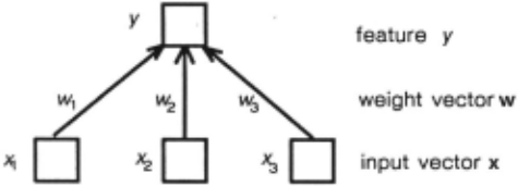
The weight vector is kept normed, i.e., after each learning step, the weight vector is divided by its length lwl = sqrt(w'+w). The complete learning rule is then
This rule is a special case of adaptation law studied by Kohonen [1984, page 103, Case 5]. As shown by Kohonen, the weight vector converges to the dominant eigenvector, i.e. , the eigenvector corresponding to the largest (dominant) eigenvalue, of the input correlation matrix E (x*x').
Since this is equally true for all weight vectors, all feature units discover the same feature, the dominant eigenvector. So this model is no serious candidate for feature discovery. However, it can be modified in several ways to perform more satisfactorily.
2.2 Competitive correlation model
One of the possible modifications is the competitive model proposed by Rumelhart and Zipser [1985] (for a more general model, see Grossberg [ 1987]) . The feature layer of this model consists of multiple feature nodes . Instead of activating each feature proportionally to the weighted input into the feature cell, only the feature unit with maximal activation, i.e., with maximal similarity ( = inner vector product) of its weight vector with the input vector "fires" and only its own weights are modified.
An obvious interpretation of the learning process in this model is that, for a given input vector, the feature with the maximal value of similarity measure (inner vector product) between the input and its currents weights learns by moving its weights toward the input vector . So competition causes each input vector to "attract" the "nearest" feature, which results in partitioning input into exclusive "clusters". Since, because of competition between features, very different inputs will probably fire different features while similar ones will fire a single common one, the system will converge to a stable state in which each feature corresponds to a cluster of input stimuli . The similarity between members within a single cluster will be significantly higher than the similarity between those of different clusters. A more formal description of this learning process is given in [Rumelhart and Zipser, 1985].
A shortcoming of this model is that some feature cells can remain inactive (i.e., they never fire because of being always outperformed by others.
A direct consequence of this behaviour is that typically very coarse features are found . The only way to refine the grain of discovered features is by increasing number of feature cells. But the more feature cells there are, the higher the probability that many of them remain inactive.
There are two proposals for remedy in [Rumelhart and Zipser, 1985] , but our analysis of them has shown that, in general case, they do not exhibit better performance than the basic competitive model [Hrycej, 1987].
There are some additional deficiencies of the competitive model :
- Features found by the competitive model are disjoint. If their number were substantially higher than two, features would be (almost) independent. But satisfying this condition cannot
always be guaranteed - on the contrary, finding only two features is very frequent (see above and Section 3.4). But then, there is, in fact, only one independent feature - the features are simply logical complements of each other.
- The representation of input by the feature layer is local since each input activates a single feature node. So the representation found does not possess advantageous properties (error correction, efficient coding, automatic generalization [Hinton et al., 1986]) of distributed representations.
- None of the features discovered by the competitive model represents a finer partitioning of others. This results directly from their disjointness. So all features are of the same hierarchical level. A hierarchical modification of such a system would be possible if additional layers were added so that clusters discovered by lower levels would be further partitioned by on higher levels. This arrangement requires an a priori structuring of the network (a tree structure) . For above reasons, such a structure would be very inefficient: successor nodes of an inactive feature node would always remain inactive, too.
- An additional drawback of this algorithm is that maximum finding is no parallel operation. (However, there are some parallel alternatives to maximization [Reggia, 1985, Chun et al. , 1987] .)
Note: The above cnt1c1sm concerns only feature-discovery properties of the competitive model. There are further valuable properties of competition, e . g., noise reduction or contour enhancement, not covered by the alternative backward-inhibition model below.
3 Backward inhibition
The drawbacks of the above competitive model result from its lack of capability to discover finer features simultaneously with coarse ones. This seems to be the very nature of competition. This section presents a concept of "backward inhibition" which copes with this problem.
3.1 Backward inhibition concept
The basis for my further reflections is the idea that more subtle features can be discovered only if strong features overshadowing them are suppressed in some way .
The implementation of this idea is very simple. After a strong feature Yi has been successfully learned, it is suppressed in the input for some time . The optimal way to suppress a feature in the next input vector is to isolate its component orthogonal to the suppressed feature, i.e., to subtract the orthogonal projection of input vector x on the feature weight vector WJ. Since the feature to be suppressed is represented by WJ with !wJI = 1, we get
with x - original input, xx - corrected input, Yi - feature unit. The suppressed feature unit will not be further activated, since
The suppression can be simulated by propagating inhibitory signal (in the size of feature activation) backwards to input units. E. g., if feature node A has been activated to activation level 2 via connections of strengths 0. 5 and 0. 3 to input nodes B and C, respectively, it inhibits nodes B and C by amounts -2*0.5=-1 and -2*0.3=0.6, respectively.
These properties of backward inhibition will be used in the next two sections for constructing feature discovery algorithms.
3.2 Eigenvectors as features
The adaptive rule of Section 2.1 discovers only the dominant eigenvector of input correlation matrix. We can use backward inhibition principle of the previous section for furhter features to converge to further eigenvectors. So all eigenvectors of input correlation matrix can be found . by successively applying backward inhibition.
Eigenvectors of a correlation matrix have some properties which make them intuitively good candidates for meaningful features :
- They extract highly correlated input lines .
- If all input lines are mutually independent, eigenvectors are unit vectors, while the dominant eigenvector corresponds to the input line with largest variance, or "the most important input feature" .
- If all input lines are completely correlated, the dominant eigenvector corresponds to the vector of input variances (or to the correlation matrix diagonal).
- If the correlation matrix can be partitioned to several diagonal submatrices corresponding to mutually independent groups of highly correlated input lines, there are eigenvectors corresponding to each of these groups.
- Eigenvectors of a correlation matrix (which is always a symmetric matrix) are orthogonal and thus independent.
- They define a linear transformation which recodes the input as completely as possible, for a given dimensionality. In other words, they explain the variability of the input in the most compact way (in the sense of main components).
So the set of all eigenvectors seems to be an appropriate feature system.
3.3 Latency time algorithm
As stated in the previous section, all eigenvectors of input correlation matrix can be found by successively applying backward inhibition. The simplest method to do this would be to use a sequential algorithm. First, it learns the dominant eigenvector, i.e. , it lets the weight vector of the first feature node converge to the dominant eigenvector. Then, it inhibits this dominant feature in the input (via orthogonal projection, see above) so that the eigenvector with the second largest eigenvalue becomes the dominant eigenvector of such a modified input, and can be in turn discovered by some other feature node, and so on until all eigenvectors have been discovered. It is, in fact, a Gram-Schmidt process for evaluation of orthogonal projections [Kohonen, 1984, page 165]. The ordering of features corresponds to descending ordering of eigenvectors by the absolute value of corresponding eigenvalues.
For all F from 1 to number of features:
learn F-th feature by the basic adaptive rule while backward-inhibiting the input by all features FF<F.
An obvious drawback (and cognitive inadequacy) of this algorithm is its sequentiality. This is, to a certain degree, an intrinsic characteristics of the problem since our adaptation rule always learns only the dominant feature . In other words, small features have to be enabled to come out of the shadow of large features by filtering large features out. This can occur only sequentially. However, control can be made parallel (or better to say local in each feature node) by the following extended activation rule applied simultaneously to all features:
- Step 1: Activate feature nodes by the basic adaptive model activation rule.
- Step 2: If the weights of a certain feature node have reached a (temporarily) stable state, this feature node performs backward inhibition of input nodes for a certain number· of cycles, the latency time.
The learning rule remains identical to that of the basic adaptive model (learning of a latent feature node is suspended during its latency time) .
For this algorithm, a criterion of weight stability is needed. A simple test of weight increment 8w for being zero, or very small; is not appropriate since input is inherently varying and thus weights never become completely stable. So an average over recent periods has to be used. I have used an exponentially weighted average of weight increment 8w over past cycles Edw!Edwabs (a ratio of average increment and average absolute value of increment) with Edw = p*Edw + (1-p)*Sw and Edwabs = p*Edwabs + (1-p) * l8w I· This ratio converges to zero if positive increments are periodically traded-off by negative increments while their absolute values may be relatively large (depending on the a-coefficient of the adaptive rule).
This feature discovery model is superior to the competitive one in several aspects:
- Eigenvectors of a correlation matrix are orthogonal (since a correlation matrix is always symmetric) and thus independent.
- The grain of feature discovery can be con trolled by latency time parameter. If latency time is short, strong features are rapidly learned while there is not enough time for weak features
- to be discovered. If the latency time is long, week features are discovered, too .
- The representation of input by the feature layer is distributed (see the following example).
- The eigenvectors being ordered by their eigenvalues, they represent a certain implicit hierarchy, as illustrated by the following example .
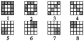
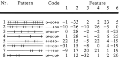
Example 1: Let us have 8 input patterns (see Figure 2) represented by 16 binary input lines. (For symmetry, -1 are substituted for zeros.) Although theoretically 16 features could be found, we will be satisfied with 6 features. Features discovered by backward inhibition algorithm are presented in Table 1 as they are contained in the patterns (the activation value of each feature multiplied by 10 is given in each feature column) . For easier orientation, an abridged code is given in the middle column . Symbol meanings are : + for feature activation > 0.7, - for feature activation < 0. 7, o otherwise.
mm v ea-=
| Nr. | Pattern | Code | Feature | ||
|---|---|---|---|---|---|
| 1 2 | 3 | 4 | 5 6 | ||
| 1 I I II I 2 II I 3 4 5 6 7 8 | II IIIII o-oo+o -1 II I II ---+oo-10 o+ooo- 0 o+ooo+ 1 ++o+o- 22 -t-oo--31 -+++o+ -9 o+-oo+ 1 | -33 -26 28 28 15 15 17 12 | 2 -10 -2 -1 -5 -8 20 -32 | 2 26 -2 -2 22 0 21 1 | 23 5 -5 0 4-25 6 25 4-19 4-19 1 19 2 20 |
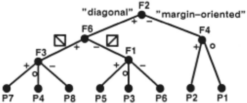
A "classification hierarchy", formed by descending order of eigenvalues is given in Figure 3. As we can see, dominant Feature 2 partitions the pateros to "diagonally oriented" (+)and "margin-oriented" (-). Those diagonally oriented are partitioned by Feature 6 to "bottom right- top left" (+) and "bottom left- top right" (-) . Features 1 and 3 measure "balancedness" of diagonal patterns .
This hierarchy is not explicit in the feature vector . However, an implicit encoding is all that is needed for input into a further associative network. Some associations can depend only on strong features like "diagonal" vers. "margin-oriented", encoded by a single feature cell F2 while weaker ones like diagonal orientation are encoded by F2 and F6 together, yet more special features by adding a further feature cell, etc., so that the actual encoding corresponds to the "path" in the hierarchy tree.
The feature system can be used to classify novel patterns, as illustrated by the following example.
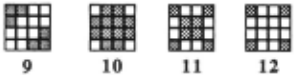
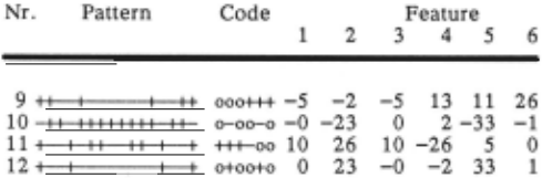
Example 2: Four novel patterns have been experimentally classified by the system (see Figure 4 and the Table 2) . Note that Pattern 9 has been classified as "bottom right - top left" and "balanced" but undecided if "margin-oriented" or "diagonal". Pattern 10 is "margin-oriented", Pattern 11 "diagonal" and "balanced" with undecided direction.
m ·· .. ·m
| Nr. | Pattern | Code | Feature | ||||
|---|---|---|---|---|---|---|---|
| 1 | 2 | 3 | 4 | 5 | 6 | ||
| 9 | ooo+++ | -5 | -2 | -5 | 13 | 11 | 26 |
| 10 II | 11111111 II o-oo-o | -0 | -23 | 0 | 2-33 | -1 | |
| 111 I | II II I I +++-oo | 10 | 26 | 10 | -26 | 5 | 0 |
| 12 | o+oo+o | 0 | 23 | -0 | -2 | 33 | 1 |
Note: With short latency times, only approximations of eigenvectors are found. Since the "residue" after suppressing "strong" eigenvectors may then substantially differ from the exact one, features corresponding to "weak" eigenvectors may substantially differ from exact eigenvectors, too. However, in all cases tested they showed very high orthogonality, so that good properties of features discovered were preserved.
3.4 Competitive algorithm
Backward inhibition can also be used to improve grain control of the competitive model of Section 2.2. After a feature unit YJ has won the competition and its weights have incrementally learned, the feature represented by its weight vector WJ is (partially) suppressed for some time:
with 0 < b < I. Parameter b controls the extent of suppression and thus the grain of feature discovery. Because of competition features do not correspond to eigenvectors.
Although this model is difficult · to treat mathematically, it can be supposed (and has been verified experimentally, see Example 3) that even weak features get their chance to attract a weight vector so that the grain of feature discovery will be refined.
Example 3: To illustrate grain control, a set of five input vectors has been taken [3,1,0,0,0]. [1,3,0,0,0]. [0,0,3,1,1], [0,0,1,3,1], and [0,0,1,1,3]. Their correlation matrix is
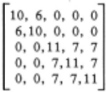
Five learning trials bave been made with five and ten feature units and b = 0.0 to 0.9 (b = 0.0 is equivalent to the original model without backward inhibition). Average numbers of active features are given in the table below.

| b | 0.0 0.1 0.2 0.3 0.4 0.5 0.6 0.7 0.8 0.9 |
| 5 units | 2.8 2.8 2.8 2.8 2.8 3.0 4.2 4.6 4.6 5.0 |
| 10 units | 3.2 3.2 3.2 3.6 3.8 4.6 4.8 - |
The 10-unit case showed poor convergence for b>0 .6, so corresponding results are not presented. It can be seen that basic competitive algorithm partitioned the patterns typically into three groups, no matter if there were five or ten feature units. The backward-inhibition-based algorithm has found, by contrast, three to five groups (five being the maximum since there are only five different input vectors), depending on the backward inhibition strength b.
4 Conclusion
Backward inhibition in a two-layer connectionist network can be used as an alternative to, or an enhancement of, the competitive feature discovery model.
The noncompetitive backward inhibition algorithm discovers features in the form of input correlation matrix eigenvectors and thus satisfies the requirements of independence, controllable grain, and distributed representation. Since the eigenvectors can be ordered by the absolute value of the corresponding eigenvalues, they form a certain "feature hierarchy".
The competitive backward inhibition algorithm operates analogically to basic competitive algorithm, but provides means for controlling the grain of feature discovery by inhibition parameter.
The advantage of backward inhibition over traditional numeric methods of cluster and variance analysis is their parallel implementation in a neural network and immediate construction of distributed representation which can be used for further processing, e . g., in a supervised-learning model.
@inproceedings{ijcai1989p27,
  title     = {Unsupervised Learning by Backward Inhibition},
  author    = {Hrycej, Tomas},
  booktitle = {Proceedings of the Eleventh International Joint Conference on
               Artificial Intelligence, {IJCAI-89}},
  publisher = {International Joint Conferences on Artificial Intelligence},
  editor    = {N. S. Sridharan},
  pages     = {170--174},
  year      = {1989},
  month     = {8},
  note      = {Parallel and Distributed Processing},
  url       = {https://ijcai.org/proceedings/1989/27},
}
TY - CPAPER TI - Unsupervised Learning by Backward Inhibition AU - Hrycej, Tomas T2 - Proceedings of the Eleventh International Joint Conference on Artificial Intelligence, IJCAI-89 PB - International Joint Conferences on Artificial Intelligence PY - 1989 SP - 170 EP - 174 UR - https://ijcai.org/proceedings/1989/27 ER -Copied
Machine-readable versions of this paper, for tools and AI agents:





