Extending the Constraint Propagation of Intervals

1 Introduction

"Constraint propagation" is often thought to be a key element in design [1, 2, 3, 4, 5, 6, 7, 8, 10), hardware debugging [11) and spatial reasoning [12). Intervals are among the most general constraints propagated; for ex­ ample , given y = 2x and 1 ::; x ::; 2, one concludes 2 ::; y ::; 4. The meaning and validity of this inference seem intuitively clear, and research attention has gener­ ally focused on its computational characteristics.

In fact, we show here that the meaning of these state­ ments and the validity of this inference, as applied to physical objects, requires more attention. More pre­ cisely, the statement 1 ::; x ::; 2 can be considered a rela­ tionship between a variable name, an interval of values, and the permissible states of the physical object being described. Reasoning about physical objects can involve at least four different kinds of such relationships. Fur­ ther, the inference shown exemplifies only one of three useful computations on equations and intervals; each of the three performs correct inferences only for appropri­ ate interval-variable relationships.

We begin. with an example demonstrating the utility of three kinds of interval propagation, then introduce four "labels" for interval-variable relationships. The bulk of the paper defines and proves the correctness of a variety of propagation inferences over "labeled intervals" . Fi­ nally, we briefly discuss the application of these ideas in a "mechanical design compiler"- a program which takes as input a schematic, specifications, and a utility function for a mechanical design, and returns a descrip­ tion detailed enough to allow construction of an optimal implementation.

·This work was done at the MIT AI Lab, with fund­ ing from the Industrial Technology Institute of Ann Arbor, Michigan, and the Office of Naval Research

1.1 An Example

Figure 1 shows graphically the governing equation, t 0 = rt;, for an ideal variable-speed mechanical transmission; here to and t; are the output and input torques, and r is the continuously variable "transmission ratio" . We use this equation to illustrate three different inferences.

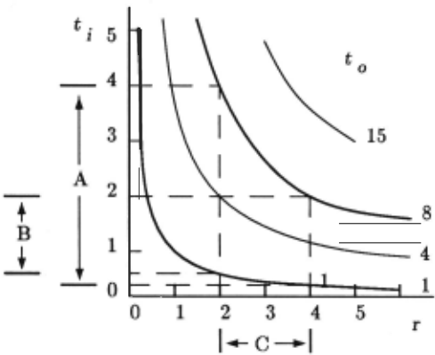
Case A: Suppose that the transmission ratio is lim­ ited to the interval from 2 to 4, and that if the output torque goes above 8 or falls to less than 1, it will damage the attached load. This seems clear enough: 2 ::; r ::; 4, and 1 ::; t 0 ::; 8. We want to pick motors which can­ not damage the load, and conclude that the input or motor torque must fall in the interval A, from 0.25 to 4; 0.25 ::; ti ::; 4. This is the usual notion of interval constraint propagation.

Case B: In contrast, suppose that under the ex­ pected operating conditions the output torque must vary throughout the interval from 1 to 8 in order to drive the load. Note that we are not saying that the output torque is limited to the interval from 1 to 8; this interval means something else. With the same limits as in case A on the transmission ratio, we conclude that the motor torque must at least vary over the interval B, that is from 0.5 to 2, or the motor will fail to drive some load. This can't be "interval constraint propagation", since it gives differ­ ent results with the same equation and interval inputs.

Case C: Now suppose that the transmission ratio is unknown, that the output torque must vary as in case B, and that the input torque is limited to the interval from 0.25 to 4. We conclude that the transmission must under some operating condition take on at least one value in the interval from 2 to 4, interval C; otherwise, at least one of the required output torques would be unattainable. "Interval constraint propagation" on 0.25 :=; t; :=; 4 and 1 :=; t 0 :=; 8 would give 0.25 :=; r :=; 32. We will show later that this inference differs from that of Case B as well. Further, the ratio is not limited to the interval from 2 to 4, nor is it required to take on every value in this interval; this interval means something different still from those we have previously encountered.

The transmission equation relates the values for vari­ ables at a particular time. However, in each case, we used the equation to draw a conclusion about the set of values a variable could or should take on. Design is a nat­ ural area of application for such reasoning, because the designer must take into account the full variety of con­ ditions under which his design must operate. Mechani­ cal designers are in fact comfortable with the reasoning of the example, but if asked to justify it can provide only intuitive arguments. We will formalize these argu­ ments, beginning by clarifying the possible relationships between variables, the states of an artifact, and intervals of values.

1.2 Assignment Intervals, and Equations

Let us suppose ourselves to be discussing an object of some sort. We describe this object using a set of vari­ able names, and suppose that it can take on various permissible states; each state assigns each variable a value from the real number line.

We need some notation. We will use S to symbolize the set of permissible states, and s for an element of S. We will write X = (x 0 2) to mean the set of assignments of values in the interval [0 2] to the variable x; x E X to mean such an assignment; and x(s) to mean the function from states to assignments of the variable x.

Assignments inherit from the real numbers such rela­ tions as<,=, min, in the obvious way. We can therefore refer to "intervals of assignments". If X is such an in­ terval, then by Xt we will always mean min(X) and by Xh, max( X). We will allow intervals to be infinite, e.g. (x 2 oo), but defer until the last section discussion of the computational implications of such intervals.

We can now introduce four kinds of statement about objects, their sets of permissible states, and intervals of assignments. We distinguish these by labeling the intervals, as in (label x Xt xh}, or just (label X}, and refer to them as labeled intervals.

That is, the permissible states assign values to x only from X; this is the interpretation given all three in­ tervals in case A. This statement is actually a predi­ cate on objects and sets of states, and could be written {[n 1 ] X)( object, S), but as we are considering only a sin­ gle object and set of states we will leave them implicit.

That is, for every assignment in X, there exists a per­ missible state of the object making the assignment. This is the interpretation given both torque intervals in Case B.

That is, there exists some assignment x in X and state s in S such that s makes the assignment x. Here we have the interpretation given the transmission ratio interval in case C.

That is, there is no state s E S such that s makes any assignment in X. As an important exception to our nor­ mal custom, we here interpret X to be an open interval. If ( none X} d X . . . fi . h h {only -} l><l an IS sem1-m mte, t en we ave 1 1 X , where X is the complement of X.

We will interpret equations describing the object as predicates on the permissible states of the object. More precisely, if the object is described using the equation G(x, y, z) = 0, then for every s E S, G(x(s), y(s), z(s)) = 0.

We impose tight restrictions on equations, discussing in [13] how these restrictions can be accommodated or loosened in practice. First, each equation must be im­ plicit, and in three variables. (If we need equations of more than three variables to describe an object, we can use intermediate variables to convert them into systems of equations.) Second, over the domain of interest the equations must satisfy the uniqueness property; that is, if G(xo, yo, z!) = 0 and G(xo, Yo, z2) = 0, then z1 = z2, and so on for permutations of variable names. Third, the domains of interest must be compatible; that is, for any permissible values of x, y there must be a per­ missible value of z satisfying the equation.

These constraints are sufficient to guarantee that the equation can be solved for each of the three variables, and that the resulting functions are strictly monotonic1. Finally, we require that these functions be continuous.

Given G(x, y, z), we will write g(x, y) to mean the associated function from assignments in x and y to as­ signments in z.

1 By strictly monotonic, for these functions of two vari­ ables, we mean that if X1 < X2 and g(x1, yl) < g(x2, Yl ), then for all x > x1, g(x, Yo)> g(x1, Yo), and so on for permutations of variable names. It can be shown for these equations that if these inequalities hold, and Y1 < Y2 and g(x1,yl) < g(x1,y2), then for all x > x1,y > y1, g(x,y) > g(x1,y1). Note that the transmission equation is strictly monotonic only over the positive reals.

2 Interval Operations and Inferences

We can now formalize a number of operations on in­ tervals and equations, asking for which permutations of labeled intervals they perform correct inferences.

2.1 Conventional Constraint Propagation

We introduce first the operation used in the introduc­ tion's Case A.

DefinitionS RANGE(G,X,Y) = {zi3x E X,3y E Y.G(x,y,z) = 0}

That is, the RANGE of the equation G with respect to the intervals of assignment X, Y is the set of assignments to the variable z such that there exist assignments in X and Y satisfying G ( x, y, z) = 0. This is of course simply the usual image of X, Y under g(x, y). The continuity of g(x, y) ensures that Z is an interval. Trivially, RANGE is commutative in the intervals; that is, RANGE( G, X, Y) = RANGE(G,Y,X).

Recall that by X! and Xh we mean min(X) and max(X) respectively; then to compute RANGE we use:

This leads to

Lemma 1 RANGE(G,X,Y) = Z =

(min(CoRNERs(G,X, Y)) max(CoRNERs(G,X, Y))] . Further, ifz1 = min(Z) = g(x;,y1), and Zh = g(xj,y2), with y 1 ,y2 E Y, then {x;,xj} = {xl,xh}·

The idea is that the maximum and minimum of a monotonic function over a pair of intervals occur at the endpoints of the intervals; further, they occur at different endpoints. The lemma of course holds for permutations of the variable names . The proof follows directly from the monotonicity and continuity of g(x, y).

For which combinations of labeled intervals does the RANGE operation produce correct inferences? We begin with the most obvious.

That is, if for every permissible state G( x , y, z) = 0 is satisfied, x( s) is in X and y( s) is in Y, then z( s) is in the image of X, Y under g(x, y). This follows directly from the definition of RANGE.

This rule expresses the inference of Case A. Recall that the output torque of the transmission should not go above 8 or below 1; ((n 1 ] t 0 1 8). The transmission ra-· · only tio could not go below 2 or above 4; (l 1 r 2 4). These, with the equation t0 = rt;, match the antecedents of Rule 1. The CoRNERS operation substitutes the end­ points of these intervals into~' returning assignments to t; of {0.5, 0.25, 4, 2}; and the RANGE operation extracts the maximum and the minimum to form {i'n 1 ] t; 0.25 4), the limits on the input torque.

We also have

Proof: By the definition of ·~'?'~ , there is some s E S such that y( s) E Y, and by the definition of (n 1 ] , x(s) is certainly in X. Then z(s) = g(x(s),y(s)) is in RANGE(G,X, Y), sot'?'~ RANGE(G,X, Y)) is satisfied.

In con-

trast, the possible rule('?'~ X)&t'?'~ Y)&G(x,y,z) = o--t'?'~ RANGE(G, X, Y)) is invalid, because the as­ signment in X and the assignment in Y need not occur simultaneously. Consider, for example, the labeled inter­ vals t'?'~ X 2 3), r'?'~ y 1 4), and equation xy - Z = 0, and the following consistent and complete set of states:

State x y z

S2

0 2 0

The rule would incorrectly imply r'?'~ Z 2 12). The same objection applies to the possible rule, ('?'~ X)&(v::J Y)--t'?'~ RANGE( G, X, Y)).

The possible rule (c;;; X)&(~· Y)&G( x, y, z) = 0---(c::; RANGE( G, X, Y)) is also invalid. Consider an object described only by (c::; x 2 3) , (~· y 1 4) , xy- z = 0. Then a state assigning x = 1, y = 6, z = 6 is permissible, and (~· Z 2 12) is false. However, let us divide the complement of X into two intervals, X1 = {xlx < min(X)}, and Xh = {xlx > max(X)} . Then, using the symbol 0 for RANGE, we have

The intuition for this rather forbidding expression is that since x ani_y can't be in X andY, they must be in overlineX andY; these complements can be divided into two intervals each; and z must be in the RANGE of one pair of such complement intervals. Hence, z cannot be in the intersection of the complements of those RANGEs. We might suppose that we could label the union of the

RANGEs with a (n 1 ]label, indicating that the assignment must fall in that union, but that union is not an interval. The intersection of the complements is an interval, be­ cause: X1, Xh, Y, and Yh are semi-infinite intervals, the RANGEs of the pairs are also semi-infinite intervals, the complements of the RANGEs are semi-infinite intervals, and the intersection of intervals is an interval.

The formal proof of Rule 3 is simple. Let the conse­ quent interval equal Z, and suppose there is some s E S such that z( s) E Z . By the antecedents, x( s) E Xi and y(s) E Yk, for j and kin {h,/}. But then z(s) is in RANGE(G, Xj, Y k), contrary to the definition of Z.

For the final rule of this section, we need:

Definition 7 INDEPENDENT( X, Y, S) if and only if for any x E X such that x = x(s!) andy E Y such that y = y(s2), with s 1 and s2 inS, then there is an s E S such that x(s) = x and y(s) = y.

As usual, we will often leave S implicit.

If for every pair x, y in X x Y there is a state making these assignments, and G is true in every state, then there is a state making every assignment in {zl3x E X,3y E Y.G(x,y,z) = 0}. We therefore have:

Rule 4

INDEPENDENT(X, Y)&("v;!; X)&C;!; Y)&G(x,y, z) 0-+(v;!! Z RANGE{G,X, Y)).

2.2 The DOMAIN Operation

We turn now to case B of the introduction, and define a partial inverse of RANGE. That is,

Definition 8

DOMAIN is partial because for some G, Z, X there is no assignment interval Y which satisfying this definition; the computation process given below readily identifies such cases. The following rules apply only when such a Y exists.

Note that since RANGE is commutative with respect to its interval arguments, DOMAIN(G, Z, X) = Y implies DOMAIN(G, Z, Y) =X.

DoMAIN has an equivalent direct definition.

Lemma 2 DoMAIN(G, Z, X) = {yi'v'x E X, 3z E Z.G(x,y,z) = 0}

Proof: Let DOMAIN( G, Z, X) = Y, and Y' = {yi'v'x E X,3z E Z.G(x,y,z) = 0}; we must show that Y = Y'. Suppose y 0 E Y. By the compatibility property, for ev­ ery x EX, there exists some zo such that G(x, y 0 , zo) = 0. But by the definition of DOMAIN, RANGE(G,X,Y) = Z, and by the definition of RANGE, Z = {zl3x EX, 3y E Y.G(x,y,z) = 0}, hence zo is in Z; that is, for every x E X there is a zo E Z such that G(x, y 0 , zo) = 0. Yo then satisfies 'v'x E X, 3z E Z.G(x, y0 , z) = 0, and Yo E Y'.

For the converse, we show first that the endpoints of Y' are in Y. Let y; = min(Y'), and let g(x1, y;) = z1, g(xh, YD = z2 .

At least one of z1, z2 must be an endpoint of Z. To see this, assume the converse; Zt < z1 < Zh, and Zt < z2 < Zh . Since g(x, y) is continuous and monotonic, we can choose some pointy' < y;, but sufficiently close to y; that Zt < g(xt,Y') < Zh and Zt < g(xh,y') < Zh. But then, z = g(x, y') E Z for all x E X , and by the definition of Y', y' E Y. This contradicts the definition of y; as min(Y'); hence, the assumption is false, and at least one of z1, z2 is an endpoint of Z .

Let Zk designate the element of { z1, z2} which is an endpoint of Z, and let Xj designate the corresponding element of {x1, xh}; that is, g(xi, y;) = zk. Lemma 1 and the uniqueness property of of G then imply that Y/ =Yt ·

We can use symmetrical reasoning to conclude that, y~ is also an endpoint of Y, then use Lemma 1 again to conclude that they are different endpoints (unless Y is a single point). Y is an interval by definition (RANGEis defined only on interval inputs), so all the assignments between y; and y~ are also in Y, and Y' = Y .

To compute DOMAIN, we rely on:

Lemma 3 JfDoMAIN(G, Z,X) = Y, then y1 = min(Y) and Yh = max(Y) are in CORNERS(g, Z, X).

Proof: RANGE(G, X, Y) = Z, so z1 and Zh are m CoRNERS(G,X, Y). Thus, for some values i and j in { l, h}, g(x;, Yj) = Zt. But then by the umque­ ness property of G, g(x;,zt) Y;, soY; is in CoRNERS( G, Z, X). Using the same reasoning with Zh and using Lemma 1, we conclude that y 1 and Yh must be in CoRNERs(G, Z , X).

We can therefore compute DoMAIN(G, Z, X) by gen­ erating each possible Yi = (y Yl Y2) where Yl, Y2 E CoRNERS( G, Z, X) and y1 ~ y2, then testing whether RANGE(G,X, yt) = Z.

To formulate our next rule, we need one more defini­ tion.

Definition 9 Let x(s1) < x < x(s2) for some s1, s2 E S; if this implies that there exists some s E S such that x = x(s), then x is STATE-CONTINUOUS.

We then have

Proof: ~ and ~ are either positive or negative throughout the domain. There are four permutations of these signs; we consider one in detail. Throughout, let Y = DOMAIN(G,Z,X). The idea is to show that there must be states making assignments of y on either side of Y.

Suppose z~ < 0, and z~ < 0. Then, g(xh,Yh) = Zt, and by the first antecedent of the rule we can choose St E S such that z(st) = Zt . By the second an­ tecedent, x(st) E X, so x(st) ~ Xh. Recall that G(x(s), y( s), z(s )) = 0 for all s E S, hence by the unique­ ness property of G, g(x(st), y(st)) = z(st). Now, as­ sume that y(st) < yh; by the assumed signs of the par­ tial derivatives, z(st) = g(x(st), y(st)) > g(x(st) , Yh) > g(xh, Yh) = z(st). The assumption must be invalid, and y(st) 2:: Yh·

Symmetrical reasoning leads to the conclusion that there is some sh E S such that y(sh) ~· y1. Then, by the STATE-CONTINUOUS assumption, for each y E [y(sh) y(st)] 2 Y, there is an s E S such that y(s) = y.

Rule 5 performs the inference of case B. Recall that we kept the limit specification on the ratio, ((n 1 ~ r 2 4}, but changed the output torque specification to require that the output torque take on every value in the interval: (v;!! t 0 1 8). The input torque is STATE-CONTINUOUS. The CoRNERS operation again substitutes the endpoints of these intervals into~. returning {0.5,0.25,4,2}. DoMAIN picks out (v;!! t; 0.5 2} by substituting into t 0 = rt; and checking the result against (to 1 8); 1 = ( .5 )(2) and 8 = (2)(4).

The STATE-CONTINUOUS assumption is physically significant. Suppose for our transmission we had (v;!! t 0 6 12}, and (t; 2 3}. Rule 5 gives (v;!! r 3 4}, which is correct for our variable speed transmission. However the requirements could be satisfied with a two­ speed geared transmission with ratios 2.9 and 4.1.

Nothing in this section proves the existence of DoMAIN(G, Z, X), and indeed this set may not ex­ ist. In Case C, for example, there is no set R of as­ signments to the ratio r such that RANGE(t 0 - rt; =

0, (t; 0.25 4}, R) = (to 1 8}. In this case, however, we can apply the next operation.

2.3 The Sufficient-Points Operation

Let us begin by extending RANGE to operate on an interval and a point (of assignment), defining RANGE(G,Y,x0 ) = RANGE(G,Y,[xo xo]). Then the SUFFICIENT-POINTS operation is defined by

Definition 10

SuFPT(G,Z,X) = {yiZ ~ RANGE(G,X,y)}

We need to show that if Y {yiZ C RANGE(G,X,y)} exists it is an interval; that is, if y1 < y2 < y 3 , and y1,y 3 E Y, then y2 E Y. Consider first the case where g~ < 0. Since Z ~ RANGE(G, X, y1) we can find some x; E X such that g(x;, y1) ~ z,. Then, g(x;, y2) < z,. Alternatively, if ~~ > 0, find x; such that g(x;,y 3 ) ~ z1, and again g(x;,y2) < z,. By symmetrical arguments there is also some Xj E X such that g(xj,y2) > Zh. Thus, Z ~ RANGE(G,X,y2), and Y2 E Y.

There is an equivalent direct definition of SuFPT.

Lemma 4 SuFPT(G, Z, X) {yi'v'z E Z, 3x E X.G(x,y,z) = 0}

Proof: Let SuFPT(G,Z,X) = Y, andY'= {yl'v'z E Z,3x E X.G(x,y,z) = 0}; we need to show that Y and Y' are equal. If y 0 E Y, let Zo = RANGE(G,X,y0) = {zl3x E X .G(x, y 0 , z) = 0}. But by the definition of Y and SuFPT, Z0 is a superset of Z, so certainly 'v'z E Z , 3x E X.G(x,y 0 , z) = 0, and Yo E Y'. Conversely, if y 0 E Y', then 'v'z E Z3x E X.G(x, y0 , z) = 0; but then Z is a subset of {zl3x E X.G(x,y0 ,z) = 0} = RANGE(G,X,y 0 ), so Yo E Y .

MAIN, we can calculate SUFFICIENT-POINTS by testing various combinations of CoRNERs(G,Z,X). We need

Lemma 5 /fSuFPT(G,Z,X) =Y, then y1 andyh are in CoRNERs(G, Z, X).

Proof: Consider first Yh = max(Y); let Z' = [z; z~) = RANGE(G,X,yh)

= [min(g(x,, Yh), g(xh, Yh)) max(g(x,, Yh), g(xh, yh))]. Then, either z1 or Zh must be an endpoint of Z'. Other­ wise, z; < z1 < zh, and z1 < Zh < z~, and since g(x, y) is continuous, we can choose some point y' > Yh suffi­ ciently close to Yh such that min(g(x1, y'), g(xh, y')) < z1 and max(g(x,,y'),g(xh,y')) > Zh. But then Z ~ RANGE(G,X,y'), andy' should also be in Y .

We can therefore find a z; which is an endpoint of both Z and Z'. By the definition of Z', G(xj, Yh, z;) = 0 for some Xj E {x,,xh}· But then Yh = g(xj,z;), and by the definitions of CoRNERS(,) Yh E CoRNERs(G, X, Z). A symmetric argument holds for y1.

We consider two inferences using SUFFICIENT­ PoiNTS. First,

Proof: Let SuFPT(G,Z,X) = Y, andY,= {YIY < min(Y)}. For y E Y1, at least one endpoint z~: of Z

is such that �(x,y,z~:) ::f 0 for any y E Y,,x E X. By the first antecedent, there is an s1 E S such that z(sl) = z~:, and by the second, x(s1) is in X, so y(sl) must be greater than max(Y,); thus, there is an s1 E S such that y(sl) ~ min(Y). By a symmetrical argument, there is an s2 E S such that y(s2) ~ max(Y). Either at least one of y( sl), y( s2) is an element of Y, or Y is included in the interval between them, in which case the STATE-CONTINUOUS assumption requires a state for every y E Y.

This rule performs the inference of Case C. We re­ quired the output torque to take on all values in an interval, (v:!l t 0 1 8}, but restricted the input torque, {[n 1 ) t; 0.25 4}. Rule 6 applies since the transmis­ sion ratio is continuously variable. CoRNERS, using r = ~ returns {4, 32, 0.25, 2}. Of these, RANGE( to = rt;, (t; 0.25 4}, r = 2) returns (t; .5 8}, which is a su­ perset of (to 1 8}. r = 4 also passes this test, but not r = 0.25 or r = 32. Hence the rule requires the transmission ratio to take on at least one value in [2 4); c~~~ r 2 4}.

For the second inference, we need another predicate on variables.

Definition 11 PARAMETER( x) if and only if there is some single assignment xo such that for all s E S, x(s) = xo.

In the design context, PARAMETER(x) implies that the value of x is fixed at manufacture.

To prove this, one applies the same reasoning as for Rule 6, then notes that since y takes on only one value, that value must be between max(Y) and min(Y).

3 Some Application Problems

The rules derived above form part of a mechanical design compiler. This program accepts specifications, a utility function, and a schematic for a mechanical design, and returns catalog numbers for an optimal implementation 2 . Implementation of the compiler involves some difficulties we avoided in the preceding discussion.

3.1 Reasoning About Sets of Artifacts

The most important complication is that while through­ out this paper we deal with representations of single ob­ jects, the compiler actually works with representations of sets of objects. [13) discusses these issues in detail; here we present only a sketch of some of the essential ideas.

Basic sets of objects are those corresponding to a par­ ticular catalog number; because of manufacturing toler­ ances, no two of these will be exactly the same. These can be described using labeled intervals; each labeled interval description is true of each object in the set.

2 The catalog numbers, together with the schematics, would usually be sufficient in the test domains to support construction by skilled mechanics. Extension to domains in which many components must be specially machined for the particular design remains a research issue.

From the basic sets, we automatically build an ab­ straction hierarchy, formulating labeled interval descrip­ tions which are true of each object in the abstracted supersets. Thus, the "cylinder" symbol in a hydraulic system schematic represents all the hydraulic cylinders in a particular catalog. Since the describing statements are true for every cylinder, the rules we have described can be used to propagate labeled intervals describing the "load", thereby inferring statements about the pumps and motors. Conflicts between these statements, and those describing the basic sets, are used to eliminate in­ appropriate basic sets. A binary search is used to find the best of the surviving implementations.

While the rules derived here remain valid, the irre­ ducibility of basic sets introduces additional rules, dis­ cussed in [13].

3.2 Relaxing the Monotonicity Assumption

Most of the equations describing mechanical artifacts are not monotonic over the real numbers. However, for a wide variety of designs it is possible to restrict values to the non-negative reals, producing strict monotonicity except perhaps at zero.

The CORNERS function may then involve divisions by zero. We extend division in the obvious ways: divisions of non-zero numbers by zero return oo; divisions and multiplications of numbers by oo return zero and oo re­ spectively. On dividing zero by zero, or multiplying zero by oo, CoRNERS returns a list including both zero and 00.

The DoMAIN operation also needs modification. Con­ sider again the transmission problem, where G is t 0 - rt; = 0. Suppose the output torque must assume ev­ ery value in the operating region ("v~ to 0 8), while the input torque is limited by (t; 0 2}. Applying Rule 5, the CoRNERS operation returns {0, oo, oo, 0, 4} . Now, only · RANGE(G,(! 1 t; 0 2},(r 0 4)) =(To 0 8), but m fact there is no need for the transmission ratio to drop to 0; any transmission ratio greater than 4 will do. For this rule, then, we modify the DoMAIN operation so that it looks for the minimal interval in r such that RANGE(G,T;, R) 2 T0 · In this case, there is no such in­ terval, and this rule make no inference. Instead, Rule 6 returns t':"~ r 4 oo) .

3.3 Performance

We discuss the expressive power of the labeled interval language and the performance of the compiler in detail in [14]. Here we remark only that the compiler has been tested on a wide variety of mechanical and hydraulic power train designs, as well a few temperature sensing systems. Some of these designs repre~ent more than a million alternative solutions; the compiler has been able to select a solution, in each case, in less than twenty min­ utes. The solutions obtained seem consistently optimal; the time required to compile designs seems to grow as the logarithm of the number of alternatives represented, or linearly as the number of equations or variables used to describe them. The compiler has not been used on designs involving feedback loops, or where dynamic (as opposed to quasi-static) performance is important.