Automated Physical Modeling

1 Introduction

Reasoning about physical systems generally involves the creation and manipulation of abstract models, normally constructed by the person studying the system. I will discuss the automatic generation of such models, as well as their manipulation and analysis. The physical sys­ tems I will focus on are mechanical devices.

An abstract model of a physical system is usually based on a set of state variables. A set of particular val­ ues for the state variables represents a particular state of the system. The model must also include a description how the state variables are related and how they change.

The values taken by state variables may be either nu­ merical quantities or qualitative symbols. The abstract models used in engineering and the physical sciences nor­ mally use state variables which take numerical values. Much of the work by artificial intelligence researchers on reasoning about physical systems has focused on mod­ els in which state variables take only qualitative values. See, e.g., [Bobrow, 1985].

Qualitative models of physical systems are often useful for reasoning in situations where the information avail­ able about the system is limited or imprecise. However, many physical systems cannot be adequately represented by qualitative models. Geometry is especially difficult to deal with qualitatively. Geometry plays a central role in the behavior of mechanical devices, so they cannot be de­ scribed by purely qualitative models, although work has been done with mixed quantitative/qualitative models for such machines. [Forbus et al., 1987, Faltings, 1987, Joskowicz, 1988, Nielsen, 1988]

*This work was supported by the NSF through grant IRI8610241. Some earlier portions were supported by ITT.

In this paper I will focus on models with numerical state variables. It is often assumed that such quanti­ tative models are not relevant to artificial intelligence because

1. We already know how to use quantitative models. Open problems are highly technical and of interest only to mathematicians.
2. The analysis of quantitative models doesn't yield results at the level needed for artificial intelligence.
3. People reason about physical situations qualitatively.

In fact, quantitative models are quite worthy of consid­ eration by AI researchers. Let us consider the objections listed above.

1. There are many open AI questions about quantita­ tive models. For example, "Where do they come from?", which is the question this paper addresses. While mathematicians and physical scientists have accumulated a wide variety of techniques for sys­ tematically analyzing such models, model creation has received little attention, probably because the techniques required are the very ones that AI spe­ cializes in. Model building is a very human activ­ ity, and involves questions like "What factors shall I neglect?", which don't have the sort of absolutely correct answer favored by the systematic techniques of the mathematical sciences.
2. In Section 7 I describe the algorithm used by my program to find a concise summary of a machine's repetitive behavior patterns. These summaries can then be used to predict the machine's long-term be­ havior. Thus the use of quantitative models and numerical simulations does not prevent the forma­ tion of concise, qualitative output of the sort one would expect from an AI program.
3. The fact that people can talk about physical situ­ ations without using numbers does not justify the conclusion that their internal reasoning methods are purely qualitative. If there is one thing AI research has taught us, it is that there is much more to hu­ man thinking than what we perceive on the surface.

Spatial and geometric reasoning, in particular, un­ questionably involve considerable information with very number-like qualities.

2 Input to the model generator

The only acceptable input for fully automated physical modeling is the actual physical system being modeled. However, dealing with this sort of input would require me to address difficult problems in robotic perception which I would rather ignore at present. Instead, my model generator takes as input a representation of the physical structure of the system to be modeled.

The representation used 1 is Constructive Solid Geom­ etry [Requicha, 1980]. In the CSG representation, each part in a machine is represented as a closed subset of three-dimensional Euclidean space which is formed by applying the Boolean set operations of union, intersec­ tion, and difference to a small set of primitive solids. For example, a square plate with a hole in it might be rep­ resented as the difference of block and a cylinder, where the block would be appropriately sized and positioned to represent the plate, and the cylinder would have the correct diameter and position so that the difference oper­ ation would create the desired hole in the plate. The ac­ tual representation is a binary tree whose internal nodes are set operations and rigid motions and whose leaves are primitive solids.

This geometric representation is supplemented with information about non-geometric physical properties such as masses, spring constants, and coefficients of fric­ tion.

3 Identification of State Variables

There is no single correct set of state variables for a physical system. Different choices of state variables are suitable for different purposes. One choice of state vari­ ables for .a mechanical device is the position and velocity of every atom of the device. Another choice is the posi­ tion and velocity of every part of the mechanism, where a part is a connected solid object. In a mechanical device, geometric constraints on the relative positions of parts in the device often allow the use of very few state vari­ ables to specify the state of a device with many parts. For example, for any position of the crankshaft in Fig­ ure 1, only one position is possible for each of the other parts. Thus the state of the device can be represented with only two state variables: the position and velocity of the crankshaft . The identification of these geomet­ ric constraints on the relative positions of parts is called kinematic analysis.

Kinematic analysis is the first step my program does in identifying state variables for mechanical devices. The algorithms used are described in detail in [Gelsey, 1987, Gelsey and McDermott, 1988, Gelsey, 1989]. Only an outline of the methods will be given here.

Kinematic analysis starts with the identification of kinematic pairs, pairs of parts which mutually constrain each other's motion. The crankshaft and frame in Fig­ ure 1 form a kinematic pair which is called a revolute pair since the only possible relative motion of the parts in the pair is rotation. Many different kinematic pairs are possible, though only a few are common.

1 I use the PADL-2 solid modeling system developed by the Production Automation Project at the University of Rochester.

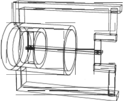
Since the only purpose of kinematic analysis is to sim­ plify the abstract model of the mechanical device by re­ ducing the number of state variables, it is not necessary to identify every kinematic pair in a mechanism. Pairs which are not identified will just result in extra state variables. For example, if the revolute pair formed by the crankshaft and the frame in Figure 1 were not rec­ ognized, then the two parts would be assigned separate state variables, and their mutual interaction would have to be computed from the basic physics of bodies in con­ tact which I will describe later in this paper.

My program identifies only very common kinematic pairs like the revolute pair, the prismatic or sliding pair, and the gear pair. These kinematic pairs are typically identified by looking for pairs of parts having subparts with matching symmetries in complementary positions. The details of the algorithm may be found in the previ­ ously cited references.

After kinematic pairs have been identified, my pro­ gram attempts to find kinematic chains, chains of parts such that each part in the chain forms a kinematic pair with its successor. A gear train is a kinematic chain, and it has the property that for any position of the first gear in the train, only one position is possible for each other gear in the train. Thus the state of an arbitrarily long gear train may be described by only two state variables: the position and velocity of the first gear in the train.

The mechanism in Figure 1 is also a kinematic chain, of a type known as a linkage. My program can analyze simple linkages like the one in Figure 1, but the gen­ eral problem of linkage analysis is quite difficult. The problem has, however, received a great deal of atten­ tion from mechanical engineers, and a survey of software which does such analysis may be found in [Fallahi and Ragsdell, 1983].

My program analyzes the mechanism in Figure 1 by determining that the axes of the three revolute pairs in the mechanism are parallel and therefore may be pro­ jected onto a plane. The projection consists of three points which determine a triangle which may be ana­ lyzed with basic trigonometry. This analysis shows that for any position of the crankshaft, only one position is possible for each of the other parts. Thus the state of the device can be represented with only two state variables: the position and velocity of the crankshaft.

My program used the results of kinematic analysis to partition the components of a mechanism into kinematic subsystems having the property that the positions of all the components of a subsystem are determined by a sin­ gle position state variable. Therefore, the total number of state variables for a mechanism will be twice the num­ ber of kinematic subsystems, since there will be one po­ sition state variable and one velocity state variable for each subsystem.

4 Neglect

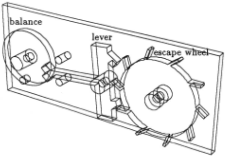
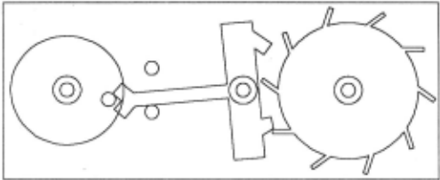
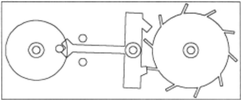
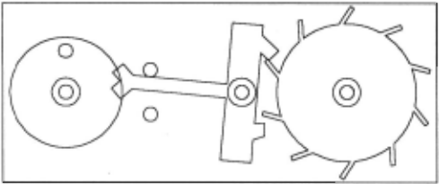
When a person creates an abstract model of a physical system, perhaps the most important issue is which as­ pects of the system should be included in the model, and which ones should be neglected. Different choices result in different abstract models. As a concrete example of such a choice, consider the clock or watch escapement mechanism displayed in Figures 2 through 5.

This mechanism forces the mainspring of the watch to unwind at a constant speed by allowing the escape wheel to advance by only one tooth for each swing of the bal­ ance, which is a harmonic oscillator [Cuss, 1952]. The cycle begins in Figure 2 with the motion of the escape wheel, which is attached to the mainspring, blocked by the lever, and the balance motionless at the top of its swing about to start moving towards the lever. In Fig­ ure 3 the balance has swung down to hit the lever. The momentum of the balance pushes the lever far enough to free the escape wheel, which then pushes both lever and balance as in Figure 4. Finally, in Figure 5, escape wheel and lever are once again locked, and the balance is at the top of its swing on the opposite side.

Figure 5: Halfway through a full cycle

The initial kinematic analysis of this mechanism finds that each of the three moving parts forms a revolute pair with the frame. No kinematic constraints on the relative motions of these pairs are found. Thus by the meth­ ods of the previous section there are six state variables: three positions and three velocities. The interesting be­ havior of the mechanism occurs when the moving parts collide and push each other. These interactions are not predicted by the initial kinematic analysis and thus must be modeled in terms of forces between the parts due to (very small) elastic deformations of parts, which there­ fore cannot be treated as perfectly rigid bodies.

A different but also valid model of the mechanism re­ sults from a decision to neglect elastic properties of the mechanism and treat each part as a rigid body. In this kinematic analysis must be used to predict the behav­ ior of the machine, but since the pairs of moving parts are only in contact part of the time, temporary kine­ matic pairs are formed and dissolved dynamically as the escapement moves. Therefore, the number of state vari­ ables changes as the mechanism runs.

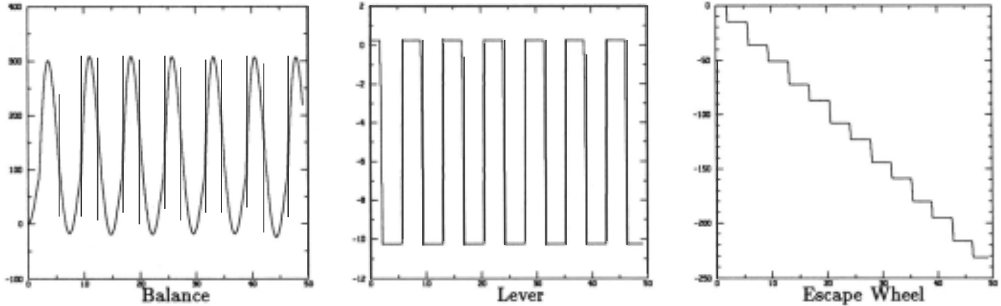
My modeling program can automatically form either of these models from the same input (described in Sec­ tion 2). They both predict the same behavior of the escapement as displayed graphically in Figure 6.

5 Computing Time Derivatives of State Variables

Identifying .state variables is only the first step in creat­ ing an abstract model of a physical system. The other essential component of the model is a description of how the values of the state variables change. The abstract models my program generates represents this informa­ tion in the form of a recipe for computing the time derivative of every state variable in the model. The full details of the algorithms used to find these "recipes" are given in [Gelsey, 1989]. Only an outline of the methods will be given here.

Let x; be the position state variable for kinematic sub­ system i, and let v; be its velocity state variable. The time derivative of x; is just v;, so the only non-trivial recipes we need to find are those for the time derivatives of the v;.

To simplify the exposition in this paper I will assume that each kinematic subsystem consists of a single kine­ matic pair. This assumption is satisfied by the first model of the escapement mechanism described in Sec­ tion 4. However, neither the second escapement model nor the mechanism in Figure 1 satisfies the assumption. They do satisfy the more general assumptions made in [Gelsey, 1989], which cover a wide selection of common machines. The general treatment, while more complex, is essentially similar to the one given here.

With this assumption,

where /; is the net force on subsystem i in the direction of motion, and m; is the mass. (In the case of revolute pairs like those in the escapement, /; ·is the net torque around the axis of rotation, and m; is the moment of inertia about that a.xis.)

The total force /; on subsystem i is

where k; is the spring constant of the spring, if any, at­ tached to subsystem i, h; is the coefficient of linear fric­ tion of subsystem i , l~c is the contact force (described below) between the two parts in contact at contact k, and a;~c is the geometric force multiplier taking the con­ tact force l~c into a force on subsystem i . ( a;1c is zero if subsystem i is not involved in contact k.)

Collisions and pushing are handled in a single uniform way. Contact forces between bodies are elastic and plas­ tic forces due to the distortion of the bodies in contact . My program uses a model of contact forces which greatly simplifies the physics involved but is still quite useful. Bodies are modeled as being rigid, but their volumes are allowed to overlap in space, and this overlap gives rise to a force. If o is the depth of overlap, the magnitude I

of the force is defined by

The contact force is basically being modeled as a lin­ ear spring with linear damping, where E is the spring constant and D is the damping coefficient. The addi­ tional factor M o in the second term on the right is there to make the force function continuous. The direction of the force is taken to be perpendicular to the surface normal at the point of contact.

A contact force contributes to v; for two different sub­ systems. 1 will be the same for both subsystems since the force acts equally though in opposite directions on each of them, but the factors a will be different.

The first step in computing the contact force between two bodies is to determine whether their positions over­ lap in space, and if so what is their depth of overlap. This computation is done by the "overlap routine", which computes the depth of overlap by applying elementary principles of geometry to primitive solids. See [Gelsey, 1989] for details. To apply Equation 3 we also need the rate of change of overlap, which has the (instantaneous) value

where v; and Vj are the velocities of the kinematic sub­ systems involved in contact k. The factors a;1c and aile are the same as those that appear in Equation 2. 2 The geometric a factors are also computed by the overlap routine.

So the final "recipe" for finding time derivatives of velocity state variables is:

1. For each kinematic subsystem i, initialize the cur­ rent value of v; to ( -k;x;-h;v;)/m; using the known constant values k;,h;, and m;, and the known cur­ rent values of the state variables x; and v;.
2. Call the overlap routine on each pair of potentially interacting primitive solids. If they overlap then
3. (a) Use Equation 4 to compute the rate of change of overlap o, using a;1c and aik computed by the overlap routine and the known current values of state variables v; and Vj.
4. (b) Use Equation 3 to compute the contact force l~c using the value of o just computed, the value of o computed by the overlap routine, and the known constant values E, D, and M.
5. (c) Add -(a;~cl~c)/m; to v; for each of the two in­ teracting subsystems (as required by equations 2 and 1).

6 Numerical Simulation

Section 4 mentions two different abstract models of the escapement mechanism, and Section 5 gives a fairly de­ tailed description of one of them. Both models describe the mechanism abstractly as a set of ordinary differential equations. These equations can be used to numerically simulate the behavior of the mechanism over an arbi­ trary time period. Figure 6 shows a plot of the results of such a simulation for the escapement mechanism.

2 That the factors are the same is basically the principle of the lever. A force at one end of a lever appears at the other end multiplied by a certain factor, and the velocity appears divided by exactly the same factor .

7 Behavior Prediction

The abstract models my program generates allow the simulation of the behavior of a physical system arbi­ trarily far in the future. However, straight simulation is an inefficient way to do long-term behavior prediction for the many physical systems, including most machines, which exhibit repetitive behavior, since simulation does not take advantage of this repetition. My program uses short, carefully controlled numerical simulations to at­ tempt to identify repetitive behavior patterns which can then be used to do long-term behavior prediction.

Instead of looking for repetition directly in state vari­ able behavior like that shown in Figure 6, my program looks at the kinetic energy of the system as a function of time. If the system has a regular behavior then so will its kinetic energy. In partic"ular the number of global minima of the kinetic energy should be the same in each behavioral cycle, and these minima should appear in the same places.

The program generates and tests hypotheses about the system's behavioral repetition. The hypothesis data structure has the following elements:

1. The duration of the system's basic behavioral pat­ tern (loop) .
2. The number of global kinetic energy minima during each loop.
3. The displacement of each state variable from one loop to the next. For example, in the behavior of the escapement mechanism as show in Figure 6, the balance and lever have the same positions in each loop, but the escape wheel position is offset by a fixed amount from one loop to the next .

Hypotheses are generated by examining the states gen­ erated by a numerical simulation which have globally minimal kinetic energy. These are simply states whose kinetic energy is both locally minimal and near the bot­ tom of the observed range of kinetic energy values. The full long-term behavior prediction algorithm is:

1. Numerically simulate the behavior of the system. As each new state is generated, identify global min­ ima of the kinetic energy.
2. Ignore the first few minima, letting the system set­ tle down. Then form a hypothesis consistent with the time and state variable values of the next two minima: the duration is the difference in their time values, the number of minima is one, and the dis­ placements are the differences in the state variable values. When the next minima is found, test the hypothesis. If it fails, form a new hypothesis consis­ tent with the new information. Repeat this process until a successful hypothesis is found.
3. Use the successful hypothesis to jump . the system forward in time, say to a time when half its total energy has been dissipated. The number of loops to jump forward by is computed from the current total energy of the system and the total energy dissipated in each loop. The jump is accomplished by apply­ ing the hypothesized displacements to the state of the system the appropriate number of times. The numerical simulation is then continued in this new situation, and the hypothesis is tested again and modified if necessary.

This algorithm has been implemented and successfully applied to the behavior shown in Figure 6. It finds a loop with two global kinetic energy minima.

8 Related Work

While there has been considerable investigation of dif­ ferent types of abstract models for physical systems [Gentner and Stevens, 1983], the problem of automat­ ically generating such models has received little atten­ tion. However, work has been done which is related to portions of my model generation process.

A great deal has been written about kinematic analysis as a human activity by people engaged in creating ab­ stract models of mechanical systems. The classic work is [Reuleaux, 1876], and a recent example is [Sub and Radcliffe, 1978]. The problem of recognizing kinematic pairs has been generally ignored in this work, since it is a relatively easy activity for humans even though it is difficult to formalize.

Several artificial intelligence researchers have inves­ tigated kinematic analysis, including Stanfill(1983] and Gelsey(1987] . Faltings(1987] and Joskowicz(1988] have attempted to formalize the problem of kinematic pair recognition by analysis of the configuration space of a mechanism.

A number of software tools exist to help mechanical engineer build abstract models of machines. A typical example is ADAMS [Dawson, 1985]. A survey of such software may be found in [Haug, 1984].

9 Conclusion

I have described a method for the automated construc­ tion of abstract models of mechanical devices. The state­ variable based models that are generated are used exten­ sively in the physical sciences, and apply to a much wider variety of physical systems than those that my program currently handles. The particular algorithms my pro­ gram uses to find recipes for time derivatives of state variables are specific to mechanics, but the central idea, the application of basic laws of physics relating state variables to their time derivatives, should make possible similar algorithms covering a considerably more varied range of physical phenomena.

Automated modeling of physical systems is an impor­ tant contribution to artificial intelligence research con­ cerning reasoning about physical systems, because any reasoning about a physical system involves an abstract model, and as long as these models are "handmade", we can't be sure how much of the reasoning which should be done by the program that manipulates the model is actually being done by the person who builds the model.