
Generating Production Rules from Decision Trees
Proceedings of the Tenth International Joint Conference on Artificial Intelligence. Knowledge Acquisition. Pages 304-306.
© 1987 International Joint Conferences on Artificial Intelligence
Abstract
Many inductive knowledge acquisition algorithms generate classifiers in the form of decision trees. This paper describes a technique for transforming such trees to small sets of production rules, a common formalism for expressing knowledge in expert systems. The method makes use of the training set of cases from which the decision tree was generated, first to generalize and assess the reliability of individual rules extracted from the tree, and subsequently to refine the collection of rules as a whole. The final set of production rules is usually both simpler than the decision tree from which it was obtained, and more accurate when classifying unseen cases. Transformation to production rules also provides a way of combining different decision trees for the same classification domain.
- Breiman, L., Friedman, J.H., Olshen, R.A. and Stone, C.J . (1984}, Classification and Regressio~ Trees, Belmont: Wadsworth.
- Bundy, A., Silver, B. and Plummer, D. (1985}, An analytical comparison of some rule-learning programs, Artificial Intelligence £1, pp 137-181.
- Finney, D.J., Latscha, R., Bennett, B.M. and Hsu, P . (1963}, Tables for Testing Significance in a 2 X 2 Contingency Table, Cambridge University Press.
- Hunt, E.B., Marin, J. and Stone, P.J. (1966), Experiments in Induction, New York: Academic Press.
- Kononenko, 1., Bratko, I. and Rollkar, E. (1984}, Experiments in automatic learning of medical diagnostic rules, Technical Report, Jozef Stefan Institute, Ljubljana, Yugoslavia.
- Michalski, R.S., Mozetil:, I., Hong, J . and Lavral:, N. (1986}, The multi-purpose incremental learning system AQ15 and its test- ing application to three medical domains, Proc. Fifth National Conference on Artificial Intelligence, Philadelphia.
- Quinlan, J.R. (1986}, Induction of decision trees, Machine Learn- ing 1, 1.
- Quinlan, J.R., Compton, P.J., Horn, K.A. and Lazarus, L. (1986}, Inductive knowledge acquisition: a case study, Proc. Second A us- tralian Conference on Applications of Expert Systems, Sydney.
- Quinlan, J .R. (1987), Simplifying decision trees, Int. Journal Man-Machine Studies, to appear.
- Snedecor, G.W. and Cochran, W.G. (1980}, Statistical Methods (7th edition), Iowa State University Press.
- Winston, P.H. (1984}, Artificial Intelligence (2nd edition), Addison- Wesley.
- Quinlan
References were extracted automatically from the PDF and may contain errors.
Full text extracted automatically from the PDF; figures, tables and equations may differ. The PDF is the version of record.
Introduction
A deci8ion tree is a simple recursive structure for expressing a sequential classification process in which a case, described by a set of attributes, is assigned to one of a disjoint set of classes. Each leaf of the tree denotes a class. An interior node denotes a test on one or more of the attributes with a subsidiary decision tree for each possible outcome of the test. To classify a case we start at the root of the tree. If this is a leaf, the case is assigned to the nominated class; if it is a test, the outcome for this case is determined and the process continued with the subsidiary tree appropriate to that outcome.
Figure 1 shows a non-trivial decision tree for one aspect of the di agnosis of thyroid disease (Quinlan, Compton, Horn and Lazarus, 1986). To simplify printing, the tree has been turned on its side. Leaves are shown in bold font, and the possible outcomes at an interior node are represented by logical expressions with equal indentation. The interpretation of the attributes and decision
· Permanent address: School of Computing Sciences, New South Wales Institute of Technology, Sydney 2007, Australia.
·· Much of the research described here was carried out at the Ar tificial Intelligence Laboratory, Massachusetts Institute of Tech nology, whose artificial intelligence research is supported in part by the Advanced Research Projects Agency of the Department of Defense under Office of Naval Research contract N00014-85K-0124. This research has also received support from the Aus tralian Research Grants Scheme and the Westinghouse Electric Corporation.
.
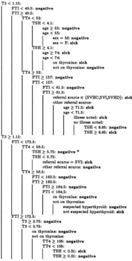
satisfied by any case classified by that leaf. For example, any case that is classified as negati11e by the asterisked leaf near the middle of Figure 1 must satisfy all the conditions
T3 ~ 1.15
FTI < 172.5
TT4 < 56.5
TSH ~ 5.75
Every leaf of a decision tree thus corresponds to a primitive pro duction rule of the form
where the X;'s are conditions and c is the class of the leaf.
At this point we make use of the training set T of cases from which the decision tree was generated in order to improve this prototype rule. Let X; be one of these conditions and let S ~ T be the set of cases that satisfy all the other conditions in the left hand side of our rule. With respect only to S, the relevance of X; to determining whether a case belongs to class c (given that the other conditions are satisfied) can be summarized by the 2 x 2 contingency table
| class c | not class c | |
|---|---|---|
| satisfies X; | 8C | 87! |
| does not satisfy X; | 8C | 8C |
where 8C is the number of these cases that satisfy X; and belong to class c, 87! is the number that satisfy X; but belong to some class other than c, and so on.
Note that 8c+8c is the number of cases in the training set T that satisfy the entire left-hand side of the rule and that 8C of them belong to the class nominated by the rule. These two numbers provide a means of estimating the accuracy or certaint11 factor of the rule. The obvious choice of setting
can be rather optimistic, especially when the numbers are small. Since for any reasonable rule sc will be larger than 8C, the use of Yates' correction for continuity (Snedecor and Cochran, 1980, pll8) gives a more reasonable estimate as
There are at least two sets of circumstances under which this condition X; should be deleted from the left-hand side of the rule. The first typically arises with disjunctiue concepts (Bundy, Silver and Plummer, 1985) in which a case belongs to a partic ular class whenever a disjunctive logical expression of the form Y V Z is satisfied. A decision tree for such a classification task might commence with a test that is relevant toY but not to Z, so the leaves associated with the disjunct Z will generate prototype rules that contain irrelevant conditions. If X; is such a condi tion, eliminating it will produce a more general rule without any decrease in accuracy, i.e. C(sc + sc, sc + sc) ~ C(8c, sc).
Secondly, the presence of x; in the left-hand side of the rule may give greater apparent accuracy, but this accuracy may de rive from chance characteristics of the training set that cannot be expected to hold for unseen cases. The algorithm used to construct the decision tree from the training set T has probably attempted to 'fit' the data, even when it is noisy or inconclusive. Under these circumstances, retaining X; can be dangerous be cause the seeming reliability of the rule can lend false confidence to a classification. There are several statistical tests that can be used to signal this state of affairs. Following a suggestion of Don ald Michie, I use Fisher's exact test (Finney, Latscha, Bennett and Hsu, 1963} to determine the significance level at which we can reject the hypothesis that X; is irrelevant to whether a case satisfying all the other conditions belongs to class c. If this level is not very small, the condition X; is deleted.
The algorithm for dropping conditions from the left-hand side of a rule can now be stated succinctly. Condition X; is ~ candidate for elimination either if its removal will not decrease the certainty factor of the rule, or if the hypothesis that X; is irrelevant cannot be rejected at the 1% level or better. So long as there are candi dates for elimination, we discard the one whose removal has the least detrimental effect on the accuracy of the rule, and continue. Of course, after any X; has been removed, the contingency tables for the remaining conditions must be recalculated.
As an illustration of the process, consider the rule above, ex tracted from Figure 1 which was in turn generated from a train ing set of 2800 cases. We focus first on the condition TT4 < 56.5. The contingency table over all cases satisfying the remaining con ditions is
| class negative | not class negative | |
|---|---|---|
| TSH < 56.5 | 12 | 0 |
| TSH > 56.5 | 141 | 0 |
so that removing this condition will increase the value of the cer tainty factor. The same holds for the condition FTI < 172.5. In the reduced rule the contingency table for the condition TSH ~ 5.75 is
| class negative | not class negative | |
|---|---|---|
| TSH < 5.75 | 168 | 0 |
| TSH ~ 5.75 | 1809 | 20 |
Even though the rule without this condition is apparently less accurate, the condition is removed because the hypothesis that it is irrelevant to whether a case in S is class negative can only be rejected at the 17% level. The remaining condition is significant at better than the 0.1% level, so the final rule from this path becomes
if T3 ~ 1.15 then class negative (99.0%)
The number of rules generated in this way is almost always smaller than the number of leaves in the decision tree. Some paths generate no rules, either because all conditions are elim inated or because the rule replicates another from a difFerent path. In this example, although the decision tree of Figure 1 has 27 leaves, the process above produces just 13 rules.
[ABide: The reader may wonder why we use the decision tree at all, instead of developing rules directly from the training set of cases. Working from the tree has two major advantages. Most interesting classification tasks involve attributes with continu· ous values which must be formed into tests by the development of appropriate threshholds (e.g. T3 < 1.15 from before). The divide-and-conquer approach commonly employed by algorithms for constructing decision trees provides a powerful and context sensitive means of coping with this otherwise complex problem. Secondly, even a long path in a decision tree typically involves only a small proportion of the possible attributes. The training set of Figure 1 uses 23 attributes to describe each case, but no path in the ·decision tree uses more than nine tests; the space of potential rules is thus shrunk from 0(2 23 ) to 0(2~) with a corresponding reduction in computational load.]
Having reduced the given decision tree to a set of plausible rules, we might judge the transformation task to have been accom plished. It seems relevant to wonder, though, how well the rules classify unseen cases, and whether some subset of the rules might be as useful as the whole set. These questions presume that there is some target production rule interpreter in the wings. The fol lowing uses an extremely simple interpreter:
To classify a case, find a rule that applies to it. If there is more than one, choose the rule with the higher certainty factor. If no rule applies, take the class by default to be the most frequent class in the training set.
Alternative and equally sensible interpreters (e.g. those that choose the most specialized applicable rule) should produce sim ilar results.
Let R be the set of production rules and T the training set of cases from which the decision tree was generated. We would like to find that subset of R which misclassified the fewest cases in T but, by analogy with the set-covering task, this is an NP problem. Instead, a heuristic algorithm is used to find a "good" subset by l!luccessively discarding single rules. ·
For any case in T and any single rule r, we look at the class to which this case would be assigned by the entire set R and the reduced set R- {r}. The advantage of r is the number of cases in T for which the correct class is given by R but not by R - { r}, less the number of cases vice versa. If the advantage of r is negative or zero, removing r from the set of production rules will not increase the number of cases in T that are misclassified. This suggests a straightforward procedure: at each step, delete from R the rule with least advantage, so long as this advantage is less than or equal to zero. The set of rules remaining at the end of this process is locally optimal to the extent that deleting any further rule will increase the number of misclassifications over T. (This may overlook, however, situations in which deleting a subset of the rules would improve performance.) The procedure usually finds a good subset of R, but is weak when the initial set of rules contains many paire of very similar rules: in this situation, most rules will have advantage 0 and so advantage is a poor basis on which to choose the rule to delete.
We saw previously that the decision tree of Figure 1 with 27 leaves gave rise to 13 production rules. The winnowing process described above reduces this set to just four rules with an average of 3.75 conditions per rule.
Accuracy
We now turn to the classification accuracy of the reduced set of rules. Since each rule was formed by eliminating conditions from a path in the tree, it tends to be over-generalized with respect to the training set. However, the relevant test of any classification mechanism is its performance on unseen cases.
| Domain | Deeision Trees | Production Rules | ||
|---|---|---|---|---|
| Average Sise (Nodes) | Average Error Rate | Average Sise (Rules) | Average Error Rate | |
| Endocrinology: hypothyroidism | 23.6 | 0.6% | 3.0 | 0.7% |
| discordant assay | 52.4 | 1.9% | 1.8 | 1.3% |
| Faulty LED digits | 92.2 | 29.0% | 15.8 | 29.8% |
| C~edit useument | 248.0 | 20.6% | 7.8 | 16.5% |
| Chess endgame | 88.0 | 11.2% | 11.6 | 9.2% |
| Disjunctive concept | 190.0 | 17.7% | 4.2 | 10.0% |
When presented with 972 unseen cases, the decision tree of Fig ure 1 misclassifies 14 of them as compared to 13 errors from the final set of four production rules above. Results from other ex periments reported in detail in (Quinlan, 1987) are summarized in Table 1. In each of six domains, ten decision trees were gen erated from a training set and their performance measured on unseen cases. Each decision tree was then transformed to a set of production rules whose accuracy was assessed on the same un seen cases. The average sizes and error rates for each domain shown in Table 1 bring out the point that the production rules are generally much simpler and sometimes more accurate than the decision tree from which they were generated.
Another advantage of transforming decision trees to production rules is their resulting modularity. There is no obvious way to combine two decision trees for the same classification task so as to generate a super-tree that is more accurate than either of its par ents. If each decision tree is converted to a set of rules, though, a composite reduced set can be produced simply by merging rules from all trees before applying the final winnowing process out lined above. This approach has been found to give encouraging results. For example, ten decision trees derived from the same training set as the tree of Figure 1, when combined in this way, yield a set of five production rules that correctly classify all but 8 of the 972 unseen cases, even though the best of the trees gives 11 errors on these same cases.
Conclusion
The conclusion of this work is that it is p088ible to re-express complex decision trees as small sets of production rules that out perform the original trees when asked to classify unseen cases. The methods outlined here also provide a way to merge differ ent decision trees for the same task, thereby obtaining another increase in accuracy.
This method for reducing the number of rules can be contrasted with the TR UNO algorithm employed in AQ15 (Michalski, Mozetil: Hong and Lavral:, 1986}. The analog of a rule in that system is a complex or conjunction of conditions &880ciated with a class. Unlike rules, complexes are exact in the sense that any case in the training set satisfying all the conditions is guaranteed to be long to the designated class. At each iteration, TRUNC discards the complex satisfied by the fewest cases in the training set until some stopping criterion is met. AQ15 uses a powerful form of partial or analogical matching to allow a case which satisfies no complex to be deemed to match the most similar complex. As a result, even though .deleting a complex cannot decrease the num ber of misclassified training cases, it may not necessarily cause an increase in this number. Interestingly, Michalski et al also report that removal of little-used complexes has been found to lead to improved classification performance on unseen cases.
Although the algorithms presented here work well, they should be capable of further improvement. Both the condition-dropping and rule-dropping processes use a hill-climbing approach which can often get stuck on a local optimum. More sophisticated search strategies should generate better individual rules and bet ter rule sets at the cost of some increase in computation.
Acknowledgements
I thank many colleagues for comments and suggestions, particu larly Wray Buntine, Jason Catlett, Bill Leech, John McDermott, Donald Michie and Ron Rivest. I am grateful to the Garvan In stitute of Medical Research, Sydney, for providing access to the thyroid data.
@inproceedings{ijcai1987p63,
  title     = {Generating Production Rules from Decision Trees},
  author    = {Quinlan, J. Ross},
  booktitle = {Proceedings of the Tenth International Joint Conference on
               Artificial Intelligence, {IJCAI-87}},
  publisher = {International Joint Conferences on Artificial Intelligence},
  editor    = {John McDermott},
  pages     = {304--306},
  year      = {1987},
  note      = {Knowledge Acquisition},
  url       = {https://ijcai.org/proceedings/1987/63},
}
TY - CPAPER TI - Generating Production Rules from Decision Trees AU - Quinlan, J. Ross T2 - Proceedings of the Tenth International Joint Conference on Artificial Intelligence, IJCAI-87 PB - International Joint Conferences on Artificial Intelligence PY - 1987 SP - 304 EP - 306 UR - https://ijcai.org/proceedings/1987/63 ER -Copied
Machine-readable versions of this paper, for tools and AI agents:





