A Quantitative Analysis of Minimal Window Search

1 Introduction

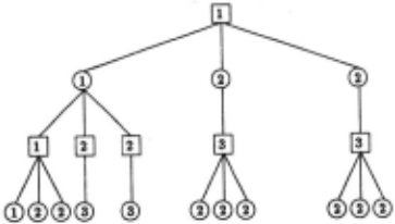
The structure most frequently used for evaluating the perfor­ mance of tree searching algorithms consists of a uniform tree of depth d and widthw .. In such regular trees th~ nodes can be cat­ egorized iiito' type cl8118es according to whether all descendants must be searched or only some of them (the so-called cut-nodes [4]). This W8ll first done by Knuth and Moore [3], who classi­ fied the nodes of optimally ordered game trees into three types (Figure 1):

• Nodes of type 1 are examined with the full-width window (-oo,+oo) . The leftmost descendant is again of type 1 and the remaining w - 1 descendants are of type 2.
• Nodes of type 2 are examined with the window (-oo,,B), which allows cut-offs. Hence, in optimally ordered trees, there exists only one descendant, which is of type 3.
• Nodes of type 3 are examined with the window (a,+oo). All w descendants are of type 2.

T .A. Marsland

Computing Science, University of Alberta Edmonton, Canada T6G 2Hl <tony@alberta.cdn>

In the following, we extend this node classification scheme to include unordered game trees and derive recursiv~ equations to compute the average performance of both the a,B-algorithin and minimal window search.

2 Analysis of Minimal Window Search

Minimal window search is hued on the 8118Umption that most of the subtrees will prove inferior to the best subtree searched so far. Having traversed the first subtree with a normal window (a,{J), the remaining subtrees are searched with the minimal window ( v, v + 1), where v represents the best available mini­ max value (e.g., the value obtained from the first selrch). If the value returned is ~ v, the subtree is indeed inferior. Only when the value returned is > v, is the initial assumption wrong and the current subtree must be re-searched with a wider win­ dow to determine its correct value. The re-search can hi! done either with an a,B-search, 811 in Scout [6,1] and Ca,B [2], or by performing a recursive self-call, 811 in NegaScout [7] and PVS [4].

integer procedure NS (position p, integer a, ,8, d); begin integer i, w, t, lo, hi; if d= 0 then return Value (p) ; (· horizon cosh) determine the successor positions: p.1, .. . ,p.w; lo +-a; hi+- ,8; for i +- 1 to w do begin t +- - NS (p.i, -hi, -lo, d- 1); if t > lo and t < fJ and i > 1 then t+- -NS(p.i , -{J, -t, d-1}; (ne-search·} lo +- max (lo, t); if lo ~ fJ then return lo; hi +-lo + 1 end; return lo end; (· cut-off ·) ( * minimal window ·)

To simplify presentation, the self-call minimal window ver­ sion of NegaScout, as shown in Figure 2, is referred to as NS. A variation, designated Nsall, invokes o.f3 to do the re-search. It is formed by replacing the corresponding line of NS with

The nodes visited when NegaScout traverses an averagely or­ dered tree are shown in Figure 3. There the node types are prefixed with an "N" , and are changed from Figure 1 because the tree is not optimal. For simplicity we initially assume that a re-search is never necessary, so Figure 3 is valid for both NS and Nsall . NegaScout starts searching the root node of type. N1 with the full window ( -oo, oo) . Since there is not yet any bet­ ter information, the root's left descendant is searched with the same full window, hence it is also of type Nl. The remaining descendants of type N 4 are searched with the minimal window (v, t1 + 1). According to our average tree assumption, these cut­ nodes have only 1 + g descendants. The first g descendants are again of type N4, whereas the {1 + g)-th descendant is of type N5, since all w descendants of this N5 node must be searched to cause the cut-off one level above.

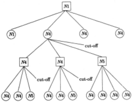
Based on Figure 3, the node dependencies can be formulated mathematically. Following an established notation [4], let k be the processing cost of an internal node and let e be the cost of evaluating a terminal node. Then N1d , the cost for searching a uniform tree of depth d and width w with 1 + g descendants at cut-nodes is given by:

N1d k + N1d-1 + (w - 1)N4d-1

N1o = e

2k + gN4d-1 + wN4d-2 for d > 1 and 0 ~ g < w

k+(1+g)e ford > 0

The consistency of these equations may be checked by observing the special case of optimally ordered game trees (i.e., the case g = 0) . By setting k = 0 {interior nodes have no cost) and e = 1 {all leaf nodes have equal cost) it is possible to show that

which is equivalent to o.f3's best case in odd-depth trees, as it should be [3]. Similarly, the consistency can be checked for even search depths.

3 Analysis of o:/3

The quantitative analysis of o.f3 is more complex, because cr{3's search process uses a window that may take any size from min­ imal to full-width. As before, we first present Figure 4, the average tree searched by o./3. Again, the root node of type A1 is searched with the full window (- oo, oo) and has descendants of type A1 and A2. The lattet are searched with a reduced window { - oo,/3) which allows cut-offs. So, only 1 + g descendants need to be searched. The leftmost A2 descendant is of type A3 and is searched with the window ( - /3,oo) . None of its descendants can be pruned, because the upper bound of the window is still infinite. However, the leaf node values gathered in this subtree establish a tight {3-bound for the search of the next g -1 nodes of type A4. Therefore, only 1 + g descendants need to be searched at this point . The rightmost A2 descendant of type AS finally returns the cut-off value, but only after all its descendants have been searched. Although they have the same number of descen­ dants, it is necessary to distinguish between nodes of type A2 and A4. The reason is that the A2 nodes are expanded with a = -oo, so that all of its left descendant's descendants must be searched. Nodes of type A4, in contrast, are searched with a narrow window (a, .B), and that allows cut-offs in all deeper tree levels.

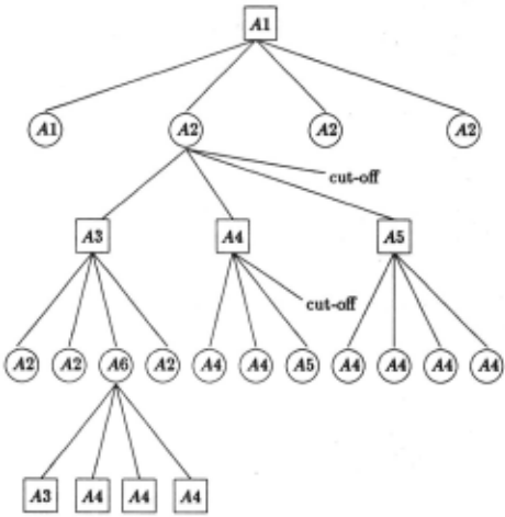
Comparing both sample trees (Figures 3 and 4), clearly a,B's lack of a finite ,8-bound at the A3 nodes causes the degraded performance. NegaScout 's minimal window search, in contrast, achieves a cut-off after 1 + g descendants have been searched at the N 4 nodes that correspond to a.B's A3 nodes. To make things worse for a.B, each A3 node has a descendant of type A6, which in turn has an A3 descendant (see Figure 4).

As for N1d, A1d (the cost for searching a uniform tree of depth d and width w with the a,B-function) may be estimated by

It is now clear that the equations for A4d and N 4d have the same form, although a.B uses only a narrow window (a, .B) rather than a minimal window (v,v+ 1).

4 Re-Search Overhead.

The model discussed so far is still too optimistic since it as­ sumes that the principal variation always lies in the leftmost path. However, it is not the location of the principal variation that is of prime importance but rather the frequency with which it changes. Assuming r principal variation changes, a,B's root node has r + 1 descendants of type A1: One lies to the left and there are r additional A1 descendants, one for each change of loc~tion. Thus for d > 0 and 0 ::; r < w,

Whenever there is a change in the principal variation, NegaScout mustdo a re-search . . This can be achieved either with a recursive self-call (as in NS) or with a call to a.B (as in Nsall). Hence for d > 0 and 0 ::; r < w we obtain two equations:

with

From Figure 3, N5d (the cost of a minimal window search that fails) may be estimated as:

For simplicity we omitted in the above equations NegaScout's "depth-2" -improvement [7], which ensures that no re-search oc­ curs when the remaining search depth is ::; 2. More precisely, for the case 0 < d ::; 2,

A similar equation can be derived for NI~ 11 .

6 Num~rical Comparison

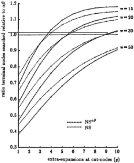
The equations just established are complex, but yield to numeri­ cal evaluation. Because there are many free variables ( d, w, g, r), and also (e, k), a variety of graphical presentations is conceivable. For example, the data in Figure 5 are obtained from trees of fixed depth d = 7, in which the principal variation changes twice at each type-1 node (r = 2) . The data-points show the search complexity as a function of g (the number of extra-expansions in cut-nodes) for various tree widths. The search complexity is given in terms of leaf-node evaluations (hence e = 1, k = 0) normalized to a,B.

Despite being degraded by two re-searches in each Nl node, the data in Figure 5 shows that both NegaScout variants outper­ form a.B in well ordered trees with low g-values. This illustrates how severely a.B is hurt by its missing .8-bound in the left part of all A2 subtrees. NegaScout, in contrast, searches these parts with a minimal window at the risk of eventually being forced to do a re-search later. The advantages of minimal window search become even more apparent in wide trees, because the overhead of the two re-searches has less influence on the overall perfor­ mance.

From Figure 5 one can see that NS is always better than Nsall if. fewer than 20% of the descendants at type 2 nodes must be expanded, even though a second re-search occurs. If more than 20% of the cut-node descendants are searched, both NegaS.cout variants are consistently poorer than a,B. So we can do without Nsall, since either pure a,B.or pure NS has the advantage.

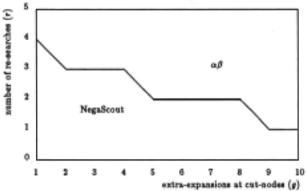
The choice between NS and cr{J depends solely on the tree ordering properties inherent in the given application. As an illustration, consider the search on trees of depth d = 7 and width w = 20, Figure 6. Clearly, those trees with gfr ratios lying below the thick line should be searched by NS, but if the tree is poorly ordered (i.e., the region above the line) cr{J should be used instead. Thus only if the re-search rate is greater than 15%, or if the principal variation is consistently in the right-half of the tree (g > w/2), does cr{J become attractive.

6 Discussion

In this paper, we presented a simple, flexible and extendible analytical model to assess the expected search time ofNegaScout and cr{J on averagely ordered trees. The model can be used to decide which of the algorithms to use in a given search task, when the ordering of the tree is known in a statistical sense.

The tree ordering properties are described in terms of g, the number of extra-expansions in cut-nodes, and r , the frequency of changes in the principal variation. In practice, r is usually small since the second-best choice prunes almost as effectively as the best. Although g, the number of extra-expansions in cut-nodes, might be as large as lf in random trees, most often heuristic information is available to sort the descendants before examina­ tion. For computer chess, average values of g in the vicinity of 1 are observed and in one study an average of 0.5 was quoted [4, p. 449] . Although the mentioned study is not strictly compara­ ble, since it used additional special-purpose pruning methods, it supports the view that the average value of g is small. Thus our model provides the theoretical basis to explain why NegaScout and PVS are superior to ~{J in practice [5] .