
The Mercator Representation of Spatial Knowledge
Proceedings of the Eighth International Joint Conference on Artificial Intelligence. Knowledge Representation. Pages 295-300.
© 1983 International Joint Conferences on Artificial Intelligence
Abstract
The MERCATOR program constructs a cognitive map from a sequence of scene descriptions. A new representation of two-dimensional geography was developed for this program. 0bjects are represented by sets of polygons; their boundaries, by sets of directed edges. The relative positions of objects are determined by connecting edges. A truth conditional semantics for this representation is presented, its strengths and weaknesses are evaluated, and it is com pared to other AI representations of shape and position.
- Davis, Ernest. Organizing Spatial Knowledge. Tech. Rept. 193, Yale University Computer Science Department, 1981.
- Davis, Ernest. Reasoning and Acquiring Geographic Knowledge. Ph.D . Th., Yale, 1983. In preparation
- Hayes, Patrick. In Defence of Logic. Proc. JJCAI 7, JJCAI, 1977.
- McDermott, Drew V. "Tarskian semantics or, no notation without denotation!" Cognitive Science 2, 3 (1978).
- McDermott, Drew V. Spatial inferences with ground, metric formulas on simple objects. Tech. Rept. 173, Yale University Computer Science Department, 1980.
References were extracted automatically from the PDF and may contain errors.
Full text extracted automatically from the PDF; figures, tables and equations may differ. The PDF is the version of record.
1 Introduction
A creature that interacts intelligently with the physical world beyond the immediate range of its senses must know the geography of its environment; that is, what objects are around it, and where they are. It must acquire this knowledge from repeated sensings of its immediate environment as it moves through space. It must make do with knowledge that is both incomplete and inexact.
I have developed a theory of how a two-dimensional cognitive map can be learned from a sequence of scene descriptions and then used. This theory has been implemented in a program called MERCATOR. In this paper, I discuss MERCATOR's representation of geographic knowledge, called a MERCATOR map. [Davis 83] describes the theory and program in full.
The MERCATOR representation has the following strengths:
- Virtually any 2-dimensional shape can be described.
- Any layout of objects can be described, including layouts where objects overlap.
- Local information can be precise, despite vagueness of global information. Specifically, it is easy to state precisely the distance between the closest faces of two objects even if the overall sizes and shapes of the objects are vaguely known or unknown.
·This research has been supported by the NSF under contract MCS7803599, an NSF Graduate Fellowship, and an ffiM Graduate , Fellowship.
maintains a world model, reflecting the true state ol the world. The MERCATOR program proper maintains a data base, representing the robot's knowledge of geography. When t he user issues an instruction for the robot to move, its mot ion is reflected in the world model by a motion simul ator, and in the data base by a motion assimilator. After moving, the vision simulator produces a scene description. This, like the data base, is expressed as a MERCATOR map.
The scene description is assimilated into the data base in a two part process. The matcher finds correspondences between the data base and the scene description. The merger adds the information in the scene description into the data base using these correspondences.
Finally, retrieval programs answer user queries using information from the data ·base. Functions have been written to determine the distance and direction between two objects, and to list the objects within a given distance of a given point.
2 MERCATOR ma.ps
Figure 2 shows a simple pastoral scene. How can we represent its two-dimensional geography!
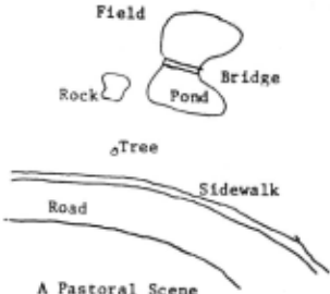
The basis elements of our representation are straight line segments. Other representations used pixels, generalized cones, reference frames , etc . However, note that figure 2 apparently captures all necessary geographic information, yet shows only the boundaries. Since the boundaries are one-dimensional, straight lines seem a natural choice. Further reasons for this choice will develop later.
Redrawing figure 2 with straight lines gives figure 3. The ··boundary of each object is represented by a set of edges connecting vertices. Thus, the boundary of the street is represented by the edges { edge (a,b), edge (b,c), edge (d,e), edge (e,f) }; the boundary of the sidewalk is { edge (d,e), edge (e,f) }; etc.
This is acceptable for a drawing, but not for a representation: it does not show the interior of the objects. Without the pond and the rock, the field would have the same boundary as the sidewalk; how could the program distinguish them! This problem is fixed in two ways in figure 4. Firstly, boundary edges are labelled with directions specifying the direction counter-clockwise around the object. Such a directed edge is called a bound. (The di agram shows the labelling only for the edges around the street but it applies to the other boundaries as well.) Thus bound (e-d) is on the boundary of the street , while bound (d-e) is on the boundary of the field. The sidewalk has boundaries in both directions on each of its edges.
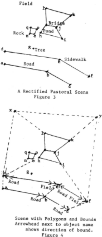
Secondly, we represent the interior of the object by polygons. The interior of the rock is covered by the polygon { polygon (n-o-p-q) } ; the interior of the field by the polygons { polygon (y-x-1-k), polygon (x-d-h-m-1), polygon (h-d-e-i), polygon (e-f-i), polygon (f-y-k-j-i) }; the interior of the sidewalk by the degenerate polygons { polygon (d-e), polygon (e-f) }; the interior of the tree by the single degenerate polygon { polygon (g)} . A complete shape description, consisting of a set of bounds and a set of polygons, is called a region.
There are, in general, many ways to break an area up into polygons. In figure 4 we could have added an addit.ional edge (e-i) in the field, and broken polygon (h-d-e f-i) into two polygons (h-d-e-i) and (e-f-i); but we are not obliged to. The system works better if the polygons are convex, but this is not necessary. It is not even strictly necessary that the polygons be discrete. Note that the fi eld, being multiply connected, cannot be described by a single polygon. The road could, in principle, be covered with a single polygon, but it is split into two convex polygons, for ease of computation.
These polygons may require edges and vertices not on the object boundary. These edges fall into two classes. /nt~rnal edges lie inside a known object, like edge (e-i) and edge (d h) . !(now/edge edges delimit the known extent of the object, like edge (a-d) and edge (x-y). It is unknown whether or not the road extends past a-d. The same distinction applies to vertices . Vertices like vertex (f) are called knowledge bounds, since it is unknown whether the sidewalk extends past. it.. A single edge may s~rve different functions for different objects; it may be a boundary edge of one and a knowledge edge of another.
The next question is how to express dimensions and rrlat.ivt> positions of objects. The easiest method would be to assign coordinates to each of the vertices. However, such precise information is usually unavailable. Allowing coord inates to be accurate only within tolerances does not help. Generally, local information is much more precise than long distance information. If all coordinates are accurate to within five feet, one cannot express the knowledge that two rocks are two feet apart, and the ten mile distance from the pond to the next village must be known accurately to within ten feet.
The diagram itself suggests the solution: local dimensions are recorded in terms of the lengths and orientations of edges connecting the vertices. Lengths and orientations are not specified precisely. Rather, we specify ranges in which they lie: the length of a-b is between 5.0 and 6.3; its orientation is between -10 and 10 degrees. We use a fixed scale and a fixed direction for measuring orientation. (See Section 5).
There is no alternative to using ranges; even if we represent these quantities as real numbers, we have to interpret them as ranges, if our system is to tolerate inaccuracy. This is particularly clear in a system which performs recognition. If I record the length of a given wall as 12.4 feet, and I see a wall which I judge to be 11.9 feet, can I say they are the same, and the discrepancy is simply the inaccuracy of the measurement! Probably. If I judge that the wall I see is 12.3 feet long, almost certainly they are the same; . if I judge that it is 6 feet long, almost cC'rtainly they are different. Eventually, I must make a biltary judgement as to whether they are the same and when I do, this will define an implicit range of seen ~alue~ which are accepted. It is simpler to use ranges from the beginning; to record in memory that the wall is 12.4 + 1- 1.2 and to have vision report that it is 11.9 + 1- 0.7. Ranges are better than point values interpreted as ranges because true ranges allow specification of both value and tolerance. An upper and lower bound are equivalent to a value and a tolerance. Since the former is easier to compute with, we will use it henceforth. Such a range is called a fu zz rang~ ; a quantity bounded by a fuzz range is a fuzziJ qu~ntit.IJ. (Fuzziness is not an attribute of the quantity, wh1ch 1s presumably real-valued; it is an attribute of our knowledge) .
All vertices must be directly or indirectly connected by edges. In figure 4, the rock and the tree are still disconnected from the other objects, so more edges must be drawn. The rock is naturally connected to the pond by edges from vertex h to vertices o and p. Generally, edges should connect nearby vertices because their relative position is more fixed and because it simplifies search procedures.
The tree is more problematical. Assume that the distance from the tree to the road is known fairly precisely -- between 10 and 15 feet -- but the position of the tree along the road is unknown. One cannot express this state of knowledge with edges which connect vertex g to the vertices of figure 4. The indeterminacy of g's parallel coordinate means that both the angle and the distance of the edge from d to g or from e to g are very fuzzy; but that would leave g's distance from the line d-e also indeterminate.
The solution is to use two edges, connected at an imaginary vertex X. The edge d-X coincides with the edge d-e and has a fuzzy length; the edge X-g is perpendicular to d-X, and has a more precise length. This arrangement of two edges is common and important enough to be defined as a separate data structure. It is called a joint from g to d along d-e, and has three fuzzy quantities: perpendicular length, from g to X; parallel length, from X to d; and parallel orientation, from X to d. The parallel orientation is always either parallel or anti-parallel to the orientation of the associated edge. (See figures 5 and 6)
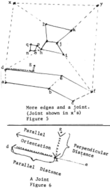
Edge lengths and orientations are less convenient than coordinates for calculations, but tolerable. The distance and direction from point a to point i in figure 4 is calculated from the lengths and orientations of the connecting edges a-d, d-h, h-i. Other quantities can likewise be calculated from the measures of connecting edges.
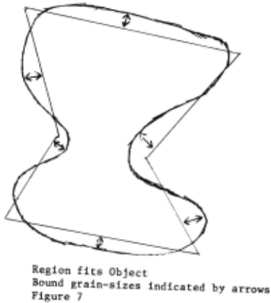
Many objects do not have straight line borders. Therefore, these representations are only approximations. It is important to define how they are approximations, and to be able to state how inaccurate a given approximation is. The measure of the inaccuracy of a region is its grain-size which is an upper bound on the distance from any point i~ the region to a point in the object. The smaller the grain Size, the better the approximation. Also, every bound in a region has a grain-size which, roughly speaking, is an upper bound on the distance from the bound to the corresponding part of the boundary. (See figure 7). A more precise definition is given in Section 3.
Sometimes it is useful to have several regions for a given object. For instance, it might be useful to have a region which showed the sidewalk as an object with thickness, or a region with more detail on the pond, in addition to the simpler regions of figure 5, which are better for quick, inaccurate calculations. We therefore separate the representation of the object as a whole from individual regions. The overall representation of the object is called a clump; it contains all the regions of the object, plus descriptions of the properties of the object, and the relations between the regions.
The description of non-geographic properties of objects is not part of our theory, and is presumably domain dependent. Its only function in MERCATOR is determining whether two clumps can refer to the same object. Therefore, we describe objects in terms of slot-filler pairs. For example a clump described as ((IS-A BRIDGE) (MATERIAL WOOD)) can match with one described ((IS-A BRIDGE) (STATE DECREPIT)) but not with ((IS-A ROAD) (MATERIAL ASPHALT)).
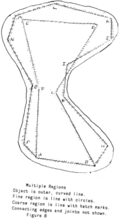
Different regions for a clump can be related to one another in three ways. Firstly, different regions may share one or more edges; in figure 8, the two regions share edge (A, B). Secondly, vertices of different edges may be connected by edges or joints. In figure 8, there is edge (K,D), (edge H,C), a joint from ito c along c-d, etc.
Thirdly, the order of the external vertices around the boundary is recorded in partial circular ordering (PCO). This is a data structure which expresses, for any three elements, whether they are in clockwise order, counter- ' clockwise order, or unordered. It is analogous to a DAG which expresses, for any two elements, whether they are in increasing order, decreasing order, or unordered. A clump with a complete outer boundary and no inner boundaries will have one PCO; otherwise, it will have a PCO for each separate section of boundary. The PCO for figure 8 is A consequence of allowing multiple regions is that the adjacency relationship becomes relative to grain-size, rather than primitive, as in many AI representations of position. At the grain-size of figure 4, for example, the road and the field share edges d-e and e-f, and are thus adjacent. Finer regions would show that they are separated by the sidewalk. This seems plausible in our domain. For planning a walk home, my house is on Lawrence Street; for walking the last ten feet, the sidewalk is next to the street; for fixing the sidewalk, there is a stone curb between the sidewalk and the street. In other domains, such as the naive physics of building towers out of blocks, adjacency is more absolute.

Finally, a map is hierarchically arranged by containment. Clumps point to their immediate containers and contents. In our example, the rock and the tree are contained in the fi eld. In a small map, this makes little difference. However, a map of realistic si1.e may show furniture inside rooms inside buildings inside blocks inside ... (See figure 9.) We shall see in section I that such organization makes calculations much more efficient. The hierarchy is a DAG, and it is assumed that its upward branching factor is small; i.e. it is almost a tree.
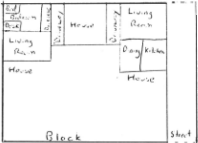
This representation is complex but complete. To review: We have clumps, representing objects; regions which approximate the shapes of objects at a given grain-size; polvgons, joints, edges, vertices, and PCOs.
3 Formal Semantics
We now formally define the meaning of a MERCATOR map in terms of a truth conditional semantics, which gives necessary and sufficient conditions that the map be a valid description of the world. Both Hayes [Hayes 77) and McDermott [McDermott 78) have argued the need for such interpretations in any system of representation. It is especially appropriate in spatial domains, where semantics are easy to define, and concepts relate in confusing ways. One might think that the informal description of the MERCATOR representation will suffice until one must answer specific questions. Then it is incomplete and ambiguous. Can the same edge represent a circular arc of coarse grain-size in one object and a very straight boundary in another! If so , how! Can we leave small objects out of a map! How small must they be! Since all our descriptions have grain-size inaccuracies, why do we need fuzz ranges!
A formal semantics is particularly necessary in the matching prohll'm, determining whether two clumps can represent the same object. There is no canonical representation of all two dimensional objects. In any representation scheme which can represent nearly all two dimensional shapes, there are shapes which can be represented more than one way. Typically, these are shapes which have no elegant representation in the scheme, like circles in the MERCATOR representation. Identifying two such shape descriptions involves more than matching identical structures; it requires consideration of how each description maps onto the object represented. The relation between description and object must therefore be defined. Two MERCATOR descriptions of a circular ring can look entirely different. One cannot write code which compares the two without a rigorous specification of what each has to do with the ring.
The semantics of MERCATOR maps are rigorously defined in [Davis 83); we will briefly sketch them here. First we define the microworld that MERCATOR maps represent. An object 0 is a closed, connected subset of R 2 (the real plane) with a boundary consisting of a finite num her of disjoint simple closed curves; equivalently, it is a subset of R 2 homeomorphic to a disk with finitely many holes. (For example, an object cannot be a figure eight.) A propertv is a function from objects to arbitrary sets. Typical properties are "color" with image set { red, blue, w bite ... } ; "style" with image set { Gothic, Georgian, Bauhaus ... } ; "is-a" with image set { robot, pond, road, .. . }. A MERCATOR map describes a set of objects with properties.
Three functions relate the MERCATOR map to the real world: REAL, COOR, and COVER. REAL maps clumps onto objects. Thus REAL (CL52) = the Empire State Building; REAL (CLIOI) = my coffee table, etc. REAL preserves containment -- i.e. if CLI contains CL2, then REAL (CLI) must contain REAL (CL2), but the converse need not be true -- and it takes clumps with stated properties onto objects with those ·properties -- i.e. if CL52 is marked as ((IS-A BUILDING) (HEIGHT VERY-HIGH)) then it is OK for REAL (CL52) to be the Empire State Building, and not OK for it to be the Atlantic Ocean.
COOR takes vertices of the map into points in the plane. Even if the point represents an object with some extent, like vertex g in figure 5, COOR (g) is a single point in the plane. COOR is extended in the natural way to take edges into line segments, joints into pairs of line segments, polygons of the map into planar polygons, and regions into unions of polygons. COOR has to satisfy the following conditions:
- For each edge e, COOR (e) has to have length and orientation within the fuzz ranges which the map specifies for e. Likewise for joints.
- For each polygon P in the map, COOR (P) must be a legitimate, non-self-intersecting polygon in the plane.
- For each region REG, every point in COOR (REG) must be no further than the grain-size of the interior of REG from the object represented by REG.
That is, the measurements given for edges and joints are correct, and regions lie on top of the objects they represent.
COVER is a fami ly of functions . COOR, as stated, maps directed edges onto line segments in the plane. However, we must relate boundary edges to the part of the object boundary that they represent. Therefore, for each directed edge b in the boundary of a region, we define a continuous function COVER 6 from COOR (b) into the object boundary. COVER 6 must satisfy the following conditions:
- For all x in COOR (b), the distance from x to COVER6 (x) must be less than the grain-size of b.
- If b and c are directed edges from the shell of region REG which meet at a vertex v, and v is a real bound of REG, then COVER 6 (COOR (v)) = COVER c (COOR (v)). This rules out situations like figure 10, which is allowed if v is a knowledge bound of REG.
- The real vertices of a clump map into the boundary of the corresponding object so as to satisfy the PCOs of the clump.
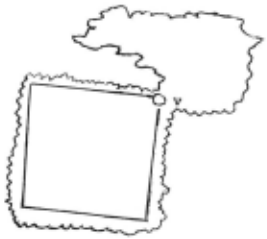
The MERCATOR map is valid if it is possible to define REAL, COOR, and COVER so as to satisfy all these conditions.
This semantics was used substantially in constructing the program. Almost all steps of the various algorithms can. be justified in terms of the semantics, u~uall.y as a deductiOn from the map(s), sometimes as a plausible mference.
4 Fuzz and grain-size
Having stated the semantics, we can clarify the dist.inction between fuzz and grain-size. Fuzz ranges are purely constraints on the COOR function. Their significance is unrelated to the real world. They wo~ld mean the same in a map without any clumps, and "':1th only edges, joints, and vertices. The! r~strict t~e poss1b~e relat ive positions of the vertices. Gram-s1ze descnbes the f1t of the geometry to the object.
In practice, fuzz measures uncertaint~ .of dimensions; grain-size measures uncertainty or com~lex1ty of shape. (See fiuure 11 ). If everything was a s1mple polygon, but di:nensions were hard to determine, there would be fuzz but no grain-size. If all dimensions were precisely known, but shapes were complex and had to be simplified, there would be grain-size but no fuzz . Grain-size is more fundamental than fuzz since it becomes necessary by the mere fact of approxim~ting shapes with polyg~ns. �rain-~i.ze can be used to express uncertainty in dimensiOn or pos1t10n, though at great loss of information. Fuzzy polygons cannot represent a circle without some grain-size inaccuracy.
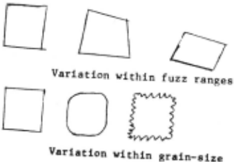
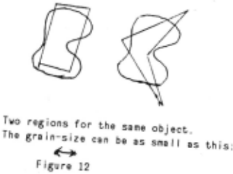
Computationally, fuzz is easic:,· to d<'~l ~ith than grain size. In comparing two regions for possible identity, for example, two regions with fuzzy edges but very fine grain size are identical only if corresponding sets of edges have overlapping fuzzes . Two shapes whose grain-size is not much smaller than the length of sides can be wildly different, yet represent the same object. (See figure 12).
6 Inadequacies of the representation
The most important gap in MERCATOR maps is that they only express the presence of an object; they cannot assert, explicitly or implicitly, an object's absence. The absence of an object from a map proves nothing; maps are not obliged to show everything, or anything, in a particular area. No map is inconsistent with the presence of any object anywhere, except that objects represented at one place in the map can't also be somewhere else in the map. Looking at a MERCATOR representation of your office, you can't say there are no rhinoceroses in the office, or even that there is reason to believe there aren't. (This answers the question posed previously how we can leave small objects out of a map. We can leave anything out of a map.)
One way to fix this gap is with completeness statements. These have the form "All obje,ts with property p larger than grain-size g inside region R have a corresponding clump in the map." For example, "All buildings larger than 0.0 in the block are shown," "All solid objects with diameter greater than one foot in the room are shown," "All wild animals in the house are shown", etc. Statements of this kind allow us to deduce that if there is no rhinoceros shown in the office, there cannot be a rhinoceros in the office. Such statements can be explicit in the data base, or implicit using default inference rules. It might, for example, be part of the semantics of a region that all objects inside it larger than twice the grain-size are represented. We have not implemented this feature in any form.
Secondly, some natural combinations of precise shape and imprecise dimensions cannot be expressed in a MERCATOR map. For example, there is no way to specify that a shape is a rectangle rather than a bizarre quadrilateral, if the lengths and orientations of all the edges are fuzzy.
The correct solution is to express lengths and orientations in relative terms. That is, length measures should be in terms like "A-B is between 2.5 and 3.0 times as long as C-D" rather than "A-B is between 4.0 and 5.0 units" or "The direction from A to B is between 0.5 to 0.6 counter clockwise of the direction from C to D" rather than "The direction from A to B is between 1.0 and 1.2 in the absolute scale." Using such facts, it is easy to state that ABCD is a rectangle. It suffices to say:
- "A-B is equal to C-D in length and orientation."
- "D-A is equal to 8-C in length and orientation."
- "A-B is perpendicular to 8-C."
InjDavis 81] and [McDermott 80] we discuss data bases for such facts , (there called "size trees" and "orientation trees"), and we show that they can be maintained effectively.
MERCATOR assumes that the robot always knows his absolute orientation, which is a very strong assumption. In fact, this problem is part of the previous one. Ideally, we would express the orientation of seen edges with respect to the current orientation of the robot, the orientation of known edges with respect to previous orientations of the robot , and the various orientations of the robot over time would be related to one another more or less fuzzily. The solution alluded to above will apply here too. There are also a less drastic solution by which the robot keeps track of his absolute orientation within fuzz bounds, which he tightens each time he matches the scene description against the known map.
Finally, the range of worlds which can be represented in a MERCATOR map is limited. It is limited to two dimensions, and to to situations where things come in well defined chunks, with perceptible boundaries. It is useless for describing a hill, a Monet, or Chinatown. These simplifications are not as restrictive as it might seem. The question is not "In what kinds of environments are these assumptions true!" -- obviously very few -- but "How much information is lost in describing a scene in these terms!", which, for many scenes, and many purposes, may not be very great.
Acknowledgements
I thank Drew McDermott for advising this research: I also thank him, together with Bianca Iano, Stan Letovsky, and David Miller, for helpful criticisms of this paper.
@inproceedings{ijcai1983p70,
  title     = {The Mercator Representation of Spatial Knowledge},
  author    = {Davis, Ernest},
  booktitle = {Proceedings of the Eighth International Joint Conference on
               Artificial Intelligence, {IJCAI-83}},
  publisher = {International Joint Conferences on Artificial Intelligence},
  editor    = {Alan Bundy},
  pages     = {295--300},
  year      = {1983},
  note      = {Knowledge Representation},
  url       = {https://ijcai.org/proceedings/1983/70},
}
TY - CPAPER TI - The Mercator Representation of Spatial Knowledge AU - Davis, Ernest T2 - Proceedings of the Eighth International Joint Conference on Artificial Intelligence, IJCAI-83 PB - International Joint Conferences on Artificial Intelligence PY - 1983 SP - 295 EP - 300 UR - https://ijcai.org/proceedings/1983/70 ER -Copied
Machine-readable versions of this paper, for tools and AI agents:





