
The Origin, Form, and Logic of Qualitative Physical Laws
Proceedings of the Eighth International Joint Conference on Artificial Intelligence. General. Pages 1158-1168.
© 1983 International Joint Conferences on Artificial Intelligence
Abstract
R~c~ntly there has been a great deal of interest within the .\rtificial lntdligcnce community in dc1cloping a qualitati1e physics (e.g .. qualitatil c process theory. em isioning. naive ph) sics) that predicts and explains the beha1 ior of mechanisms in qualitative terms . The goals for the qualitati1e physics are (1} to be far simpler than classical physics and yet retain all the important distinctions (e.g .. state, oscillation. gain. momentum) without invoking the mathematics of continuously var.ing quantities and differential equations. (2} to produce causal accounts of physical mechanisms that are easy to understand, and (3} to provide the foundations for common-sense models for the next generation of expert systems. This paper consists of three parts. First. we present a framework for understanding and unifying the various approaches :o qualitative physics as well >~S posing certain criteria that such a physics should satisfy. Second, we compare and contrast three approaches to qualitative physics. Finally, we explore the use of proof as explanation and the role reducrio ad absurdum plays in qualitative arguments in physics.
- es," to appear in Fonna/ Theories of the Common-Sense World, edited by Jerry Hobbes and Bob Moore, Ablex, 1983.
- de Kleer, J. and J.S.Brown, "Assumptions and Ambigu ities in Mechanis- tic Mental Models," to appear in Mental Models, edited by D. Gentner and A. S. Stevens, Erlbaum, 1983.
- de Kleer, 1. and J.S. Brown, "Mental Models of Physical Mechanisms and their Acquisition," in Cognitive Skills and their Acquisition, edited
- by J.R. Anderson, Erlbaum, 1981.
- de Kleer, J., "Causal and Teleological Reasoning in Circuit Recog- nition," Artificial Intelligence Laboratory, TR-529, Cambridge: M.I.T., 1979.
- Forbus, K.D. and A. Stevens, "Using Qualitative Simulation to Gen- erate Explanations," Report No. 4490, Bolt Beranek and Newman Inc., 1981.
- Forbus, K.D., "Qualitative Process Theory," Artificial Intelligence Laboratory, AIM-664, Cambridge: M.I.T., 1982.
- Forbus, K.D., "Qualitative Reasoning about Physical Processes," Proce~ dings of the Seventh International Joint Conference on Artificial Intelligence, pp. 326-330, 1981. IJCAI
- Ha)es. P.J .. "The 1\aive Physics Manifesto."" in E.xperr Sysrems in rhe Microe/ecrronic Age. edit~d by D. t-.1ichie. Edinburgh University Press. 1979.
- Kuipers. B .. '"Getting the Emisionment Right."' Proceedings of rhe Narional Conference on Arrificia/ lnrelligence. pp. 209-212, 1982.
- Kuipers, B .. ••commonsense Reasoning About Causality: Deriving Behavior from Structure," Tufts University Working Papers in Cogni- tive Science No. 18. May 1982.
- Williams. M .. J. Hollan and A. Stevens,"Human Reasoning about a Simple Physical System," to appear in A/ental Models, edited by D.Gentner and A.S. Stevens, Erlbaum, 1983.
References were extracted automatically from the PDF and may contain errors.
Full text extracted automatically from the PDF; figures, tables and equations may differ. The PDF is the version of record.
.\BSTR.\CT
R~c~ntly there has been a great deal of interest within the .\rtificial lntdligcnce community in dc1cloping a qualitati1e physics (e.g .. qualitatil c process theory. em isioning. naive ph) sics) that predicts and explains the beha1 ior of mechanisms in qualitative terms. The goals for the qualitati1e physics are (1} to be far simpler than classical physics and yet retain all the important distinctions (e.g .. state, oscil lation. gain. momentum) without invoking the mathematics of con tinuously var.ing quantities and differential equations. (2} to produce causal accounts of physical mechanisms that are easy to understand, and (3} to provide the foundations for common-sense models for the next generation of expert systems. This paper consists of three parts. First. we present a framework for understanding and unifying the various approaches :o qualitative physics as well >~S posing certain criteria that such a physics should satisfy. Second, we compare and contrast three approaches to qualitative physics. Finally, we explore the use of proof as explanation and the role reducrio ad absurdum plays in qualitative arguments in physics.
WHY QUALITATIYE PHYSICS IS IMPORTANT
The motivations for developing a qualitative physics stem from outstanding problems in psychology, education, artificial intelligence, and physics. Humans appear to use a qualitative causal calculus in reasoning about the behavior of their physical environment. Judging from the kinds of explanations humans give, this calculus is quite different from the classical physics taught in classrooms. This raises questions as to what this (naive) physics is like, and how it helps one to reason about the physical world.
In classical physics the crucial distinctions for characterizing physi cal change are defined within a nonrnechanistic framework and thus they are difficult to ground in common experience. Qualitative physics provides an alternate and simpler way of arriving at the same concep tions and distinctions and thus provides a simpler pedagogical basis for educating students about physical mechanisms.
Artificial intelligence and (especially) its subfield of expert systems are producing very sophisticated programs capable of solving tasks
THE ORIGIN, FORM AND LOGIC OF QUALITATIVE PHYSICAL LAWS
Johan de Kkcr and John Seely Brown
XEROX PARC Cognitive and I nsmtctional Sciences 3333 Coyote Hill Road Palo Alto. California 94304
which require cxtensi1e human expertise. A commonly recognilcd failing of such systems is their extremely narrow range of expertise and their inability to recognitc when J probkm posed to them is outside this range of expertise. In other words, they have no common-sense. _usually expert systems cannot soh·e simpler versions of the problems they are designed to solve. The lacking common-sense can be supplied by qualitative reasoning.
Analysis of a physical situation can be divided into three roughly sequential activities. The first is modeling the structure of the physical system in some kind mathematical formalism. The second is solving the model thus produced. The third is interpreting the results of the solution process for the physical system. These three activities are highly interrelated as each depends critically on the mathematical formalism being used.
COI\1MONALITIES: VARJABLE, VALUE, AND CONSTRAINT
In a conventional quantitative physics, modeling is in terms of variables which potentially can take any real value. Qualitative physics adopts the notion of variable, but describes each variable with a small finite number of distinctions. Many significant variables in physics models are derivatives. In qualitative physics. the value of a derivative is usually described by "+","0", or "-," corresponding to whether the variable is increasing, unchanging. or decreasing. Arithmetic on these values is straight-forward: if X and Y are both negative, so is X+ Y, if X is zero and Y is negative, X+ Y is negative, if X is positive and Y is negative, the sign of X + Y is undetermined, etc.
This value set is not sufficient for variables which are not deriva tives. Typically a variable has distinguished values abo1·e or below which behavior is radically different. For example, a string breaks if its tensicln is too high (T > T .\IA.\ ) . Thus. a network of inequalities rna~ exist ~unong the 1ariabks. As the number of such inequalities is finite. the set of all inequalities di1 ides the potential 1alws for each 1ariable into a finite set of iiHerYals on the real line. Each such region corresponds to a particular qualitative ,·alue. Thus in the case of the string. T has two values: below T.lt.·L\ and above TAux.
TI1e choice of distinguished Yalues for 1·ariables is a serious problem. Clearly, 0 is an importam distinguished Yalue for deriYatiYes, but what is the origin of the distinguished 1alues for other variables? One possible scheme is to choose simple symbolic Yocabularies (e.g., TALL VERY"TALL etc.). As Forbus[82] points out, such arbitrarily chosen schemes are based on the particular situation being analyzed. It is always possible to choose just the "right" symbolic vocabulary for each variable after analyzing the situation. This produces a model, a solution, and an interpretation which have the appearance of cogency, but are, in fact. vacuous as the appearance of success depends on the comext-sensitiYe choice of distinguished values. For this reason, the distinguished values for variables must be derived from the structure of the situation in some relatively direct way (e.g., TMAX ).
Can qualitative physics be based on simultations?
As there are strong similarities between a qualitative analysis of a situation and a qualitative simulation of a situation it might seem natural to cast the qualitative physical laws as production rules for simulations. Although the result of such an analysis (i.e., a causal account) might be expressed in such a manner, effons to formalize such a physics have all ended up using constraim systems for representing physical laws in modeling. Here v.:e consider three reasons for this decision in the context of Figure 1.
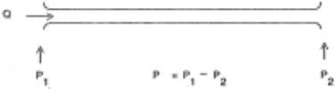
A succinctness problem. A panial model for a pipe might be: "if the pressure across the pipe increases. the flow through the pipe increases." This suggests encod!ng laws for the behavior of a pipe with production rules such as: "if dP = + then dQ = +-" This is a very seductive option. but it actually introduces needless complications. Such productions Yiolate succinctness: a complete model for the pipe requirt'S fi1e other such productions (if dP = 0 then dQ = 0. if dP =- then dQ = - . if dQ = + then dP =+.etc.). I11ese other productions Cclmain essemially the same infcmnation. hence there is needless duplication. For more complex componcms. the duplication is even more serious.
A semantics problem. The "then .. in each of these mles is misleading because it in1plies the passage of time where there is none. It is a 1·iolation of physical law for the pr~ssure across the pipe to rise with eYen a momentary delay in the rate of flow through the pipe. The rise in pressure across the pipe must co-occur with a rise in rate of flow. The law for the pipe is better phrased as: "if it is discovered that the pressure across the pipe is rising. then it must also be the case that the rate of flow through the pipe is rising."
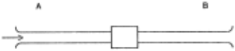
A completeness and locality problem. Even if one recognizes this semantics problem of "then." an analysis of overall device behavior can be incomplete. Suppose one executes the laws as a conventional production system would: i.e .. repetitively mn every production-law whose left-hand side matches and assen the corresponding right-hand side. This process does not discover what happens in the situation illustrated in Figure 2. Two pipes are connected in series, the right hand end is held at constant pressure and the pressure at the left-hand side is increased (by some external force). In this case the pressure at the point where the pipes join must be rising, but there is no production that states this. A production for a pipe triggers only if the pressure across it or the flow through it is known. Ip this example, no flow is known and only the pressure at one end of each of the pipes is known. Therefore no production triggers. However, by reasoning over the productions, an indirect argument can be constmcted for why the pressure at the joint rises. Assume the pressure at the joint is constant, then a production for pipe B asserts that there is no change in flow through it. Hence there is no flow change through pipe A and another production produces that the pressure across pipe A is constant. This contradicts the fact that the pressure across the combined two-pipe system is increasing, hence the pressure at the joint cannot be constant. A similar argument shows the pressure at the joint cannot be dropping, hence it must be rising.
The particular difficulty here is not so much whether productions are an adequate representation, but that "simulation-like" interpreta tions of them are inadequate. It is here that qualitatil'e physics diverges from qualitative simulations. This example shows that if the physical laws are local, as they must be, simulation is an incomplete inference mechanism. (Clearly one could add a production for two pipes linked to each other but this approach eventually explodes and has limited explanatory power as all such stmctural combinations might require explicit mles.)
Because of these three problems most current versions of qualita til"e physics choose to describe laws as constraints. and view solving as a constraint-satisfaction task. The complete constraint model for a pipe is "any change in pressure across the pipe is proportional to any -;hange of flow rate through it" or simply dP = dQ. Such constraints have these advantages: (1) they are succinct, (2) they do not suggest passage of time, (3) complete solution methods based on constraint-satisfaction are directly available, and (4) constraints can support both imperative interpretations (they can be executed) and assertional interpretations (i.e., they can be reasoned over).
THE FORM OF THE LAWS
The preceding views of value, variable, and constraint essentially are shared among the qualitative physics of ourselves, of Kuipers, and of Forbus. The major differences concern the precise statements of the constraint Jaws and how they are derived from the physical structure. The central organizing principle for Forbus is the notion of process, for Kuipers the notion of constraint, and for ourselves the notion of physical component.
Qualitative Process Theory according to Forbus
A process is the basic source of change in physical situations. Heating, flowing, moving, expanding, boiling. stretching are all ex amples of physical processes in qualitative process theory. The rules of the process indicate (1) under what conditions the process holds (called quantity conditions), (2) the relations it imposes among vari ables, and (3) the influences it imposes on the variables. The physical situation presented in Figure 4a can be described by the heat-flow process. The quantity condition for the heat-flow process is that the temperature of the source of the heat is greater than the temperature of the destination of the heat The relations state that (1) heat flows from the source to the destination and (2) this flow rate is qualitatively proportional to the difference in temperature between the source and the destination. The heat-flow rate negati vely influences the heat of the source and positively influences the heat of the destination. This process is represcnt~d qualitatiwly (from [Forbus 82]) as shown in Figure 3.
process heat-flow
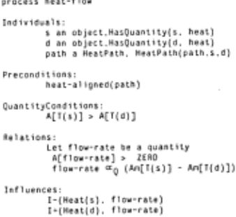
Unlike a relation, an influence does not place a complete constraint upon variable values. The influence I- (H eat(s), flow-rate) states that flow-rate negatively influences the heat of the source, but other processes, such as burning. may also influence the amount of heat The complete constraint on the amount of heat in the source is determined by sum of all the influences of an the processes which reference it: in general ?, = L:P'"""es I(x, q). The +. -, 0 value of ?, can be determined using the qualitative arithmetic of Table l.
Qua/itacive modeling according to Kuipers
Kuipers employs five types of individual constraints among vari ables: arithmetic, functional , derivative, inequality, and conditional. The arithmetic constraint asserts that the values of the variables must ha\'e the indicated relationship within any time-point. The functional constraint Y = M+(x) asserts that Y is a strictly increasing (or decreasing if M-) function of X. The derivative constraint Y = f, X asserts that at any time-point, Y is the rate of change of X . The inequality and conditional constraints specify conditions under which some other constraint holds.
The "causal structure description" indicates each of the constraints and variables of the model. Figure 4a (from (Kuipers 82)) is a pictorial descriotion of a simple physical system with its "structural" description. The system consists of a container of gas at temperature T which is heated by a Bunsen burner at temperature T5 . The rate of flow of heat into the gas is a strictly increasing function of the difference t.T between the two temperatures, with t.T = 0 corresponding to no heat flow in to the gas.
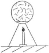
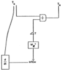
To solve this model a qualitative simulation is done by propagat ing +. -, o values (using Table l) and inequalities (using con train! propagation) in order to obtain values for all of the variables. Additional analysis rules are required to determine the behavior of the siruation over time, but no augmentation to the model is required to do so.
Envisioning according to de Kleer and Brown
We take the view that a device consists of physically distinct parts connected together. The goal is to draw inferences about the behavior of the composite device solely from laws governing the behaviors of its parts.
Our central modeling primitive is the qualitative differential equa tion, called a confluence, which acts as a constraint on the variables and derivati\·es associated with components. For example, the qualitative behavior of a valve (Figure 5) is expressed by: dP + dA- dQ = 0. In this equation, Q is the flow through the valve, P is the pressure across the valve, A is the area available for flow, and dQ, dA, and dP represent changes in Q, A, and P. The confluence represents multiple competing influences: the change in area positively influences flow rate and negatively influences pressure, the change in pressure positively influences flow rate, etc. The same variable can appear in many confluences and thus can be influenced in many different ways.
f~tch confluence must be sJtisfi~d indiddually. Thus if th~ area is increasing but the flov. remains constant. the pressure must decrease no matter what the oth~r influences on the pressure arc.
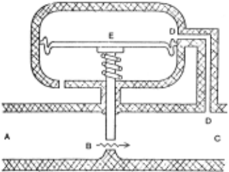
A single set of confluences often cannot characterize the behavior of a component over its entire operating range. In such cases this range must be divided into subregions, each characterized by a different component state in which different confluences apply. For example, the behavior of the valve when it is completely open is quite different from that when it is completely closed.
The full model for the valve is:
The behavior within each state is described by different confluences. The state is specified by inequality conditions among the variables which indicate the region within which the confluences are valid. Somewhat surprising has been the realization that this notion of state, which is a convenience in the analytical regime, rums out to be a logical necessity in the qualitative regime.
Comparison
Another commonality among the different approaches is the use of conditional laws -laws that hold only if some other conditions are meL Quantity conditions. state specifications. and inequalities/conditions are all similar in that some other constraints become relevant if they hold.
Although qualitative process theory and envisioning are very similar in that both rely on an underlying formulation in terms of constraints, the form of their rules are radically different. Qualitative process theory is process-centered, while envisioning is component centered. As a consequence, information that is locally available in one theor} IS dtsmbutcd 10 the other and ncc vcrs.1. In this sense th~y arc duals to each other. In qualitatil e process theory. the influences of diverse processes must b~ gathered to dctcnninc a constraint on a 1ariable. In em·isioning. each conflu~nce of a component places a necessary constraint on the variables it references. Of course. the same variable may participate in the confluences of models of neighboring components.
The situation of Figure 4a can be modeled using three com ponents: a Bunsen burner. a container. and a connection path. The heat·flow path obeys the confluence law. dH = TD- Ts (i .e .. the flow of heat through the path is proportional to the temperature difference between the two ends of the pipe). In envisioning, the presence of heat flow follows as a consequence of component laws.
Kuipers' theory avoids taking a position on this issue as its initial description is already a set of constraints over the entire device as opposed to a confluence which is a constraint describing a single component.
THE ORIGIN OF THE MODEL OF THE SITUATION
Given a model for a composite device, one must answer the question of where the components. processes, or constraints of the overall device model come from. Even if the resulting predictions are accurate and explanations are acceptable, unless some criteria are placed on obtaining this composite model, much of the success might be attributable to idiosyncratic choices. What good is a qualitative physics if it provides no information linking the model to the physical situation? Said differently, going from a physical situation to a differential equation is where · most of the work gets done in physics, i.e., in constructing a cross section of the physical situation that manifests the underlying mechanism which in tum forms the basis for formulating the differential equation. Doing physics is deriving the equations from the physical situation. Doing mathematics is solving the resulting equations.
Kuipers' theory has absolutely nothing to say to this issue. His model of the physical situation requires a list of constraints bearing no connection to the description of the physical structure. He places no criteria upon what patterns of constraints are allowable or physically possil}le. He only provides a representation of qualitative differential equations and solution methods for them - it is a qualitative math ematics, not a qualitative physics. To call the constraint diagram of Figure 4b a "causal structure description" is misleading as it is neither causal nor related to physical structure.
A qualitative physics must provide a set of heuristics and tech niques for constructing (composite) device models. It is unreasonable \> expect a complete procedure for constructing device models, but it is retsonable to expect principles to guide their construction. Qualitative proc..-ss tllcor! meets U11s cntcnon 10 111 o 11 ays. First. each model builder must draw upon a shared common 1·ocal;ntbry of abstract processes 11 hich arc used to model all situations. Second. additional reStrictions are placed on the fonn of a process in order that it bear close resemblance to the intuitive idea of physical process (e.g .. boil ing. freezing. expanding). Each process must explicitly describe the indi1·iduals about which the process is concerned (processes interact by sharing individuals). Furthermore. the process must indicate precon ditions under which it is valid. For example. the heat-flow process is valid only if the source and destination of heat are aligned such that the two indil'iduals are in thermal contact. A model builder is not free to invent an idiosyncratic process which must be introduced to produce an adequate account of some situation.
For emisioning, the (composite) device model is derived from the device topology and a predetermined vocabulary of component _models. The device topology describes the structure of the composite device indicating the physically distinguishable parts of the device and how they are connected. The device model is constructed by modeling each of the components of the device topology, but the model for each indiYidual component may only reference variables of other components which are adjacent to it through some connection. Envisioning has an advantage over qualitatiYe process theory because it builds on an explicit. objective description of the structure of the composite device. In qualitative process theory the modeler is saddled with the task of identifying abstract processes which are operative in the physical situation. Envisioning has the additional advantage that it explicitly indicates how each piece of the physical structure causally contributes to the overall functioning of the system - a critical propeny for a variety of tasks.
EXPLANATION AND THE ROLE OF RAA
The previous sections have provided an introduction and a brief oven·iew of the field of qualitative physics. In this section we focus on one particular issue. We explore the use of logical proof as explanation for qualitative predictions. We do not do this because we especially espouse logical proof as an explanatory vehicle, but rather we use it as a foil to bring two subtle problems into focus. That is, we want to provide a framework for analyzing kinds of explanations for how physical devices function. First, the logical framework provides a mode of explanation such that each explanation is compelling (i.e., every result follows by necessity) and the set of all such explanations can be shown to be exhaustive. As such it provides a standard by which to evaluate other alternatives. Second, and more in1portant. by framing explanation in a natural deduction system we have been able to isolate how and why purely causal explanations cannot account for all physical mechanisms. This sets the stage for a new definition of causality.
Tht· .\lode/ for !he Pressure Regu/mor
The specific confluences governing !he behavior of !he device can be constructed from !he description of the srrucwre of !he de1·ice and !he library of component models. The confluences for !he pressure regulator (Figure 5) form seven confluences in eight 1·ariables. The pressure regulator has only two components. each of which is modeled by one confluence. The remaining confluences describe !he behavior of the material flowing within !he components and their interconnections. We state all the confluences in terms of !he particular variables for !he pressure regulator (Figure 6). The subscripts on !he variables indicate which terminals and conduits of !he device topology !he variable refers to.
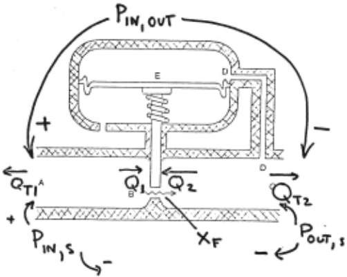
The confluence for !he valve is
where P1s.oL·r is !he pressure drop from input to output, Q#I(VJ) is !he flow from terminal #1 into !he valve, and dXF is !he position of !he valve control. The confluence for the pressure sensor is
wher~ ?0 1 r. s is !he pressure at the output of the pressure regulator. ·n1e area a1ailablc for flLlW must 1ar! in1ersely 11ith output pres sure. Th~ rcnuining confluences wncern cons~nation of material and definition of pressure:
The flow through !he load connected to !he pressure regulator is proportional to !he pressure across it:
Prediction
To determine !he behavior, assignments of+. 0, and - to !he variables must be found !hat satisfy !he confluences of !he device. Given an input signal of dP1,v.s = +. !here is only one set of assignments values to !he variables !hat satisfies !he confluences:
dQn =
dQT2 = +
dQ#2(V J) =
dQ#l (VJ) = +
dXF=
dPnv,OUT = +
dPour,s = +
In English: The flow out of !he input of !he pressure regulator is decreasing (equivalently, !he flow into !he input of !he pressure regulator is increasing); !he flow out of !he output of !he pressure regulator is increasing: !he flow into !he output-side of !he valve is decreasing; !he flow into !he input-side of !he valve is increasing; !he area available for flow is decreasing; !he pressure across !he valve is increasing; !he output pressure is rising. Note !hat !here is a certain amount of arbitrariness in choice of sign conventions, but we systematically choose !he sign comentions such !hat flows are always into components away from conduits and flows are always out of global de1·ice connections.
These solutions can be obtained through various techniques (e.g., constraint satisfaction). Our purpose here is to provide a framework for analyzing kinds of explanations for how physical systems function.
Proofs as Explanations
"'aive physics is concerned with both prediction and explanation. An explanation con~ists of a sequence of statements, each dependent on swtemems earh<.?r m the sequence. 1 he enure srquence somehow accounts for the predicted bclm ior. Cmcial to this r<.?search is the r<.?cognition that an explanation is not a post-hoc rationaliLation for a prediction. rather it has predictiYe power in its own right: e1 ery syntactically 1alid explanation must describe a possible prediction. An explanation must be compelling and lea1·e no doubt as to the validity of its conclusions. This single requirement for explanation establishes a very strong connection between prediction and explanation. As an explanation consists of a sequence of statements it should, in principle. be possible to do prediction by generating all sequences of statements and testing to see which are 1·alid explanations. Of course. the converse is also true: we can define an explanation as the execution trace of whatever algorithm is used to make the prediction. Although this form of explanation certainly meets the criterion. explanations are intended to communicate information and thus they also should be succinct. One structure that meets the two criteria of compellingness and succinctness is logical proof.
An explanation consists of a sequence of statements E1 , E2, ... , where each statement is justified by statements previous in the se quence. The confluences provided by the component models and the input signal(s) provide the givens. The justifications are in terms of simple logical inference steps on the statements. The explanation is expressed as a proof in a natural deduction system [Suppes 57). In this system the theorem is the prediction and the proof is the explanation; thus a theory of "explanation" (or at least a taxonomy of different kinds of structures for explanation) can be discovered from examining the different kinds of proof structures.
Each line of the proof consists of a line number (so it can be referenced}, a statement, a justification of the statement, and a set of premises upon which the statement depends. The following is part of an explanation for why the valve starts to close (i.e., dXF = -) when the valve is opening.
| [I) dXF + dPoc"T,S = 0 | Given | {} |
| [2) dQn - dPour,s = 0 | Given | {} |
| [3) dQ#2(VI) + dQn = 0 | Given | {} |
| [4) dQ#I(VI) + dQ#2(VI) = 0 | Given | {} |
| [5] dQ#I(VI) = + | Premise | {5} |
| [6) dQ#2(VI) =- | Substitution 5, 4 | {5} |
| [7) dQn = + | Substitution 6, 3 | {5} |
| [8) dPocr ,s = + | Substitution 7, 2 | {5} |
| [9) dXF=- | Substitution 8, 1 | {5} |
This explanation-proof can be rendered into English as follows (the givens have been put in a more natural order). Suppose the flow into the input-side of the valve is increasing [5). As the valve conserves material [4), the flow into the output-side of the valve must be decreasing [6). As no material is gained or lost in the connection from the output of the Yahe to the output of the pressur<.? r<.?gulator [3]. the flow out of the output-side of the pressure regulator is increasing [7). As the flow through the load is proportional to the pressure across it [2). this results in an increased outpllt pressure [8]. '111is output pressure is sensed [1], and the area available for flow is reduced (9].
(All the explanation-proofs presented in this paper are constructed automatically by our program. i.e .. lines 1-9 are a 1·erbatim output. The English text is added by us for expository purposes. Our program, EN\'ISION. takes a description of the physical structure of the device and a library of component models. constructs a model for the overall device, solves the model thereby making predictions, and produces explanations as illustrated above.)
This particular explanation used three kinds of justifications cor responding to the application of three inference rules. "Given" indi cates that the statement is a confluence obtained from the models or from the applied input signal. "Substitution n1 , ··. , n;, m" indicates that value assignments n1 , ·· · , n, a're substituted into confluence m . "Premise" indicates an arbitrary unsubstantiated assignment introduced to make the explanation go through. Note that lines 1 - 9 do not explain the necessity of dXF = - because the underlying premise [5) dQ-~; 1 (vi ) =+has not been substantiated. In a conventional natural deduction system one would derive the statement
[9') CP 9,5 {} by conditional proof. Namely, if it can be shown that dQ#I(VtJ = + then dXF = -. In English: suppose the flow into the input-side of the valve is increasing, then the area available for flow is reduced. However, from the three inference rules there is no way to show that dQt; 1(v 11 = + necessarily follows.
The Crucial Role of Indirect Proof
It can, however, be shown that dQ#I(VI) = + by arguing that dQ#l(I' IJ =J + is contradictory and thus by reductio ad absurdum dQ#t(VIJ = +. namely by an indirect proof. As a qualitative variable can have only three values it is sufficient to show that dQ#l(VI) = 0 is contradictory and dQ#I(VI ) = - is contradictory. We need to introduce three new types of inference rules. "Unique Value n , m" indicates that the assignments of lines n and m directly contradict each other. "RAA n , m" indicates the contradictions of line n and m force an assignment by reductio ad absurdum. "Discharge n, m 1 , ..· , m;" indicates that the assignments of lines m 1, ... , m ; can be used to remove unsubstantiated premises from line n. "RAA'' and "Discharge" derive directly from natural deduction systems. "Unique Value" is a short hand for a lemma derived from a simple axiomatization of equality: every 1·ariable must have one and only one value. More formally:
\\"it.h t.his additional infcr,;-ntial machinery, i.e .. t.hc machinery of indirect proof. Y.e can proceed to prove or explain why t.he 1 alve will stan to close when t.he input pressure is increased. The remaining twenty-one steps of t.he proof for t.hc pressure regulator's behavior discharge t.he assumption t.hat dQ#11 , ·1J = +. Note that some of the confluences only play a role in the discharging, hence they do not appear in the proof until these steps.
| [10] dP1s.on - dQ#l(n) + dXp = 0 | Given {} |
| [11] dPJN,ou'r + dPot'T.s- dPJ.-..•,s = 0 Given | {} |
| [12] dQ#l(VlJ = 0 | {12} Premise |
| (13) dQ#2(Vl) = 0 | {12} Substitution 12,4 |
| [14] dQT2 = 0 | {12} Substitution 13,3 |
| (15) dPouT,S = 0 | {12} Substitution 14,2 |
| (16) dPIN,S = + | {} Given |
| (17) dPJN ,OUT = + | Substitution 16, 15, 11 {12} |
| [18]dXp =- | Substitution 12, 17, 10 {12} |
| [19] dXp = 0 | Substitution 15, 1 {12} |
| [20] False | Unique Value 18, 19 {12} |
| [21) dQ#l(Vl ) = | Premise { 21} |
| (22) dQ#2(Vl) = + | Substitution 21,4 {21} |
| [23] dQT2 =- | Substitution 22,3 {21} |
| (24) dPouT,S = | Substitution 23,2 {21} |
| (25) dPIN ,OUT = + | Substitution 16, 24, 11 {21} |
| [26]dXp = | Substitution 21, 25,10 {21} |
| [27]dXp = + | Substitution 24, 1 {21} |
| [28] False | Unique Value 26, 27 {21} |
| [29) dQ#l(Vl) = + | RAA 28,20 {} |
| [30]dXp =- | Discharge 9, 29 {} |
In English: Suppose the flow into the input-side of the valve were not increasing, but unchanging [12]. Then by conservation [4], the flow into the output-side of the valve is also unchanging [13], and again by conservation [3], the output flow of the pressure regulator is unchanging [15]. As flow through the load is proponional to the pressure across it [2], there is no output pressure change [15]. Now, we are given that the pressure regulator input pressure is rising [16], and since the difference of pressure regulator input and output pressures appears across the valve [11], the increased input pressure appears across the valve [17]. In the situation where there is no change in flow and there is an increase in pressure there must [10] be a decrease in area available for flow through the valve [18]. On the other hand, if there is no change in output pressure there cannot be [1] a change in area [19]. Thus assuming that the flow is unchanging leads to a contradiction [20]; the flow cannot be unchanging. The only possibility that remains is that the flow into the valve is decreasing [21]. By an identical line of argunwn. [21-28]. that assumption also leads to a contradiction. Hcnc"'. by indirect argument the flow into the input-side of the valve is increasing [29]. llms. the area ;l\ ailable for flow is decreasing [30].
The intuitiw notion of a compelling explanation can now be stated precisely, namely one which docs not depend on any undischarged premises. In the pre1ious example. [30] dXp = - must necessarily follow. Qualitative analysis can sometimes be ambiguous. thus it is not always possible to discharge all the premtses. Consider the case where the input pressure is lower than the output pressure. In this situation all the confluences remain the same except the valve confluence:
This is the same confluence as line [10] in the above explanation-proof, except that the sign of the area change is in vened. This is because of the behavioral characteristic of the pressure regulator that an increase in area available for flow always reduces the absolute value of the pressure drop. If the pressure drop is a positive value, an increase in area decreases it to zero (as in the previous analysis). If the pressure drop is a negative value, an increase in area increases it to zero. The resulting analysis is ambiguous, in principle, and no unique value can be found for dXp . The following are explanation-proofs for the two possible values for dXF.
| [1] d)(F + dPouT,S = 0 | Given | {} |
| [2] dQT2- dPouT,S = 0 | Given | {} |
| [3] dQ#2(V1) + dQT2 = 0 | Given | {} |
| (4] dQ#l(Vl) + dQ#2(Vl) = 0 | Given | {} |
| [5) dQ#l(Vl) =- | Premise | {5} |
| [6] dQ#2(V1) = + | Substitution 5, 4 | {5} |
| [7) dQT2 =- | Substitution 6, 3 | {5} |
| [8) dPouT,S =- | Substitution 7, 2 | {5} |
| [9] dXF=+ | Substitution 8, 1 | {5} |
| [1] dXF + dPouT,S = 0 | Given | {} |
| [2) dQT2- dPov T,S = 0 | Given | {} |
| [3) dQ#2(Vl) + dQT2 = 0 | Given | {} |
| (4) dQ#l (V l) + dQ#2(Vl) = 0 | Given | {} |
| [5) dQ#! (V!) = + | Premise | {5} |
| [6) dQ#2(Vl ) =- | Substitution 5, 4 | {5} |
| [7) dQT2 = + | Substitution 6, 3 | {5} |
| [8] dPon,s = + | Substitution 7, 2 | {5} |
| [9) dXF=- | Substitution 8, 1 | {5} |
(We could also show that dXv ~ 0.) The point is that no pmnf exists for discharging or cnmradicting !he assumptions of either line 5. II "hen rhe <111<1/.rsis is ambiguc' IIS. cu·llpellillg e.lpl,l!Wfions CJIIIIOI. in principle. exis1.
Allowing assumptions in explanation opens !he floodgates to an extremely serious problem: arbitrarily many exp!Jnations are now syntactically valid and appear plausible. By allowing unsubstantiated premises we, in effect, allow a proof for A:JB to be an explanation for B. If A is false. !he implication is still valid but the proof may provide no information about !he validity or !he plausibility of B. It is impossible to tell from an explanation alone whether or not its outstanding assumptions can be ruled out. It is hard to show !hat a particular premise will not be discharged or contradicted. For example, in !he above two proofs no further sequence of statements can contradict or discharge !he remaining assumptions (without, of course, introducing other assumptions which themselves cannot be discharged, etc.). In general, to show !hat !he theorem A:JB and its explanation-proof is !he best result achievable requires showing !hat A is neither true nor false. If A were true, we would have a compelling explanation forB alone. If A were false, A:JB is trivially true. However, one cannot tell from a proof for A:JB whether it is also possible to determine !he validity of A. An even more difficult result to explain is !hat !he given set of interpretations is complete, i.e., !here exist no other theorems of !he form A:JB for a behaviorally different B and for which A cannot be proved to be true or false.
For most devices, no explanation exists within !he calculus which does not include premises. However, !he local ambiguity can often be resolved because !he device's behavior exhibits no global ambiguity (i.e., !he premise can often be discharged). Thus !here are two fun damentally different roles for assumptions which are locally indistin guishable. An assumption either can represent a global ambiguity or can be a temporary construction to enable an explanation-proof to go through. The latter type of local ambiguity arises because !he system is simultaneous.
Proof as Explanation
..:Jbere are four undesirable characteristics of explanation-proof !hat are symptomatic of its inadequacy as a theory of explanation: (1) !he introduction of premises into an explanation is unmotivated and ar bitrary, (2) indirect proofs are intuitively unsatisfying, (3) explanation proofs are non-unique, and (4) explanation-proofs can be causally invened. We explore each of these in detail.
Premises are introduced because of local ambiguity but can often be resolved because !he device's behavior exhibits no global ambiguity. Even so, !he premise must be introduced arbitrarily in !he explanation proof (and later discharged). Although this might seem plausible if the de\ icc's beha\·ior were globally ambiguous. it seems questionable !hat exp!Jnations for unambiguous beha\ior shtluld be so arbitrary. r\s the choice of assumptitln is not dctennined. usually many different assumptions will independemly lead to valid explanations for the same behavior.
Indirect arguments are counterintuiti\ e. One would like explana tions to consist of steps. each describing correct behavior which follows by applying a component model rule to functionings described in ear lier steps (something like !he proof but without RAA). Neither is the case for indirect explanation-proofs. The steps may refer to hypotheti cal functionings which do not actually occur and a justification might be RAA. Indirect proofs explain a consequence by showing !hat all alternative consequences do not happen. and thus cannot establish a simple relationship between a cause and its effect.
The same conclusion can have many proofs. none of which can be identified as !he "correct" one .. Hence, !here may be multiple explanation-proofs for a device's functioning. Although it might make sense in a few cases to have two or three explanations for how a device behaves. it makes little sense to have multiple explanations for a device's behavior at the same grain size of analysis. Remember !hat we are considering explanations for !he same behavior in terms of !he same component models. Multiple explanations can sometimes arise because !he confluences are redundant, but more commonly arise due to !he arbitrary choice of premise. In our framework !here usually exist an extremely large number of syntactically acceptable valid proofs, but it is straightforward to eliminate most of !hem by employing a minimality condition. However, !here still remain roughly fifteen different explanations for !he pressure regulator's unambiguous behavior, corresponding to !he different minimal combinations of premises !hat can be introduced to analyze the device. A particularly undesirable one is obtained by introducing premises about dXF. The explanation is now totally indirect.
| (1) dXF =- | Premise | {1} |
|---|---|---|
| [2) dQ#2(Vl) + dQn = 0 | Given | {} |
| [3) dPu-: ,OUT- dQ#l(Vl) + dXF = 0 | Given | {} |
| [4) dPnv,ouT + dPouT, s - dP1.v,s = 0 | Given | {} |
| [5) dXF + dPor..:T,S = 0 | Given | {} |
| [6) dXF = 0 | Premise | {6} |
| [7) dPouT,S = 0 | Substitution 6, 5 | {6} |
| [8) dhv,s = + | Given | {} |
| [9) dh~·.ouT = + | Substitution 8, 7, 4 | {6} |
| [10) dQ#l(Vlj = + | Substitution 6, 9, 3 | {6} |
| [ll) dQ#l(Vl) + dQ#2(V2) = 0 | Given | {} |
| (12) dQ#2(Vlj =- | Substitution 10, 11 | {6} |
| [13) dQn = + | Substitution 12, 2 | {6} |
| [14) dQn- dPour,s = 0 | Given | {} |
| [15] dQn = 0 | Substitmion 7, 14 {6} |
| [16] False | Unique Yalue 15, 13 {6} |
| [17] d.Xv =- | Premise {17} |
| [IS] dPm r.s =- | Substitution 17, 5 {17} |
| [19] dhv.on = + | Substitmion 8, 18, 4 {17} |
| [20] dQ#l(\'ll = + | Substitution 17, 19,3 {17} |
| [21] dQ#2[1ll = - | Substitution 20, 11 {17} |
| [22] dQT2 = + | Substitmion 21,2 {17} |
| [23] dQT2 =- | Substitution 18, 14 {17} |
| [24] False | Unique \'alue 23, 22 {16} |
| (25] d.XF = '- | RAA 24,16 {} |
In English: Suppose the area available for flow were not changing [6]. Then the sensor does not [5] sense any output pressure change [7). As the input pressure is rising, this rise must (4) appear across the valve [9]. If the area available for flow is unchanging and the pressure across the valve is increasing the flow into the input-side of the valve must [3) be increasing [10). As the valve conserves material [11] the flow into the output-side of the valve is decreasing [12] and as the output connection also conserves material (2), the flow out of the output of the pressure regulator must be increasing [13]. However, it was shown earlier that the output pressure was unchanging (7]. and hence there can be (14) no change in flow through the load [15]. This contradiction shows that the area available for flow must be changing [16]. On the other hand. suppose the area available for flow is increasing [17), then the sensor must sense [5] a decrease in output pressure [18]. An increase in input pressure and a decrease in output pressure dictate (4) the valve pressure decrease [19]. By the same argument used in [10-13], the .flow out of the pressure regulator increases. However, it was shown earlier that the output pressure was decreasing [18). and hence there can be (14] no increase in flow through the load [23]. This contradiction shows that the area available for flow cannot be increasing [24). As the area must be changing, and cannot be decreasing, it must be increasing [25).
In this explanation we see another undesirable feature of indirect explanations: the steps in the explanation do not follow any notion of causal order. The explanation proceeds from output to input The key problem is that the explanation-proof explains why the device must behave not how it behaves - the latter is the task of causal explanations.
R.\A and Causality
Our goal is to have accounts that are both compelling and causal. Without using RAA, the proof cannot be the basis for compelling explanations, yet the presence of RAA and indirect argument is antithetical to causality. Recognizing RAA as the central issue suggests SC\Cral kinds solutions to this tension (sec [de Klecr & Brown 83] for d~tails). Consider the process b) "'hich the pans of th~ d~\ice int~ract to produce the overall beha\iOr of the de\·icc. 'lbcse interactions must all be local. i.e .. each part is on I) abl~ to int~ract "ith its physically adjacent neighbor. On the other hand. RAA is non-local. !bus the device itself apparently achie\·cs its functioning without invoking anything like RAA.
Why introduce the notion of causality when the predictiYe theory seems sufficient? We want a theory which describes how devices function and not just what their bchaYior is. The confluences and the solution algorithms say nothing about how the de\·ice functions. Instead the confluences arc merely constraints on behavior and the algorithm a method of constraint satisfaction. The explanation-proof says little about how the device functions, and instead only proves that the particular instance of constraint satisfaction is correct. In short, it embodies the epistemological principle "There is a reason for everything" at the expense of the ontological principle "Everything has a cause."
Let us rniew the reasons why we care about creating causal accounts. both from an ontological and an epistemological perspec tive. Causality as a theory of how deYices function provides many advantages. Because it is a theory of how the device achieves its beha\·ior rather than just what its behavior is, it proYides an ontologi cally justified connection between the structure of the device and its functioning. It is now possible to ask what functional changes result from hypothetical structural changes (a task imponant in troubleshoot ing). Without causality this question could only hope to be answered by a total reanalysis. Clbus causality provides an approach to solving the frame problem [Hayes 79].) Because it describes how behavior is achieved by the device, more information about the behavior can be uncovered. For example, feedback, which alters the behavior of the device, can only be recognized definitively by understanding how the device achieves its behavior. This is because feedback is a propeny of functioning, not of behavior. Since causality is a universal mode of understanding functioning, it provides a medium by which device functioning can be explained, whether as a designer to a user, a teacher to a student, etc. Finally, since causal accounts are so universally adopted as the model of understanding, most common pat terns of causal interactions around indi\·idual components have been identified and abstracted often forming the basic elements of techni cal vocabularies. These abstractions arc a kind of canonical form which can be used as indices into other knowledge about component behavior. For example, knowing that a transistor is operating in the mode in which the base is the causal input and the collector the causal output (called the common-emitter configuration) tells us imponant things about that circuit's gain and frequency response - things that would be impossible to derive from the prediction of the qualitative behavior alone.
Devices function causally, yet the necessity for RAA rules out simple definitions of causal it). Our approach is to relax the definition of causality slightly still retaining the basic idea of not losing complete ness or compellingness. yet avoiding the necessity for RAA. A detailed discussion of our solution is beyond the scope of this paper: here we outline our general approach. Superficially, the necessity for RAA results from the particular confluences used to model the behavior of components. There turns out to be no way to change the confluences (nor their fonn) to satisfy locality and fidelity while avoiding the use of RAA. We must look more closely at the physical principles used to derive the component models: The central thernwdynamical principle that underlies the construction of almost any model is that of quasistatic approximation: the device is presumed always to be infinitesmally near equilibrium. Of course, if the device behavior is examined in sufficient detail, one must observe some non-equilibrium intermediate states, otherwise the device could not change state! The equilibirium models are a result of making a quasi static approximation that behavior of short enough duration is irrelevant and can be ignored. Equilibrium models cannot, in principle, describe how change happens. Thus, the neces sity of RAA and the consequent inability to produce causal accounts stems from having made quasistatic assumptions in the modeling of component behaviors. Avoiding quasistatic approximations altogether does not help as one must then refine the grain size of the analysis to the point (perhaps to the quantum mechanical level at which other problems come to the fore) that the resulting complexity becomes un manageable and largely irrelevant. Our solution is to leave the original models unchanged, but define a new kind of causality (which we call mythical causality) that describes the trajectory of non-equilbrium states the device goes through before in re-achieves a situation where the quasistatic models are valid. The component laws for mythical causality are based on a careful procedural interpretation of the equi librium constraint laws. Trajectories through non-equilibrium states are accounted for by viewing the device's components as performing a simple computation.
A POSSIBLE CONFUSION
A central concern of qualitative physics is the production of causal accounts for behavior. One must be extremely careful to distinguish the process by which an analysis tool produces a causal account, and the process by which the physical device produces its behavior. The former need not be "causal." We have not discussed in any detail how the constraints of the device model are solved. to produce the causal account. Given the constraint nature of the rules one might not expect any close correspondence between the process of solving the constraints and the process which achieves the physical behavior.
It is interesting to speculate on how close a correspondence might be achievable between these two process<-s. The discussion of the two pipe example (Figure 2) illustrates how the analysis process and the causal process can diverge. In conventional quantitative physics, the analysis process might involve the solving of the differential equations of a field to determine the movement of an electron. while the causal process is the manner by which the electron. itself, decides in which direction to move.
In our ongoing research we are attempting to bring the analysis and the causal processes into close correspondence. If a complete cor respondence could be achieved (perhaps through the use of negotiation in mythical time) then we would have the basis for a new branch of physics. one in which the flow of information plays as fundamental a role as the flow of energy and momentum.
ACKNOWLEDGMENTS
We thank Danny Bobrow for his suggestions concerning earlier drafts. Kurt Van Lehn. Steve Locke and Dan Russell provided many helpful comments.
BIBLIOGRAPHY
de Kleer, 1. and J.S. Brown, "A Qualitative Physics based on Confluenc es," to appear in Fonna/ Theories of the Common-Sense World, edited by Jerry Hobbes and Bob Moore, Ablex, 1983.
de Kleer, J. and J.S.Brown, "Assumptions and Ambiguities in Mechanis tic Mental Models," to appear in Mental Models, edited by D. Gentner and A. S. Stevens, Erlbaum, 1983.
de Kleer, 1. and J.S. Brown, "Mental Models of Physical Mechanisms and their Acquisition," in Cognitive Skills and their Acquisition, edited by J.R. Anderson, Erlbaum, 1981.
de Kleer, J., "Causal and Teleological Reasoning in Circuit Recog nition," Artificial Intelligence Laboratory, TR-529, Cambridge: M.I.T., 1979.
Forbus, K.D. and A. Stevens, "Using Qualitative Simulation to Gen erate Explanations," Report No. 4490, Bolt Beranek and Newman Inc., 1981.
Forbus, K.D., "Qualitative Process Theory," Artificial Intelligence Laboratory, AIM-664, Cambridge: M.I.T., 1982.
Forbus, K.D., "Qualitative Reasoning about Physical Processes," Proce~ dings of the Seventh International Joint Conference on Artificial Intelligence, pp. 326-330, 1981.
Ha)es. P.J .. "The 1\aive Physics Manifesto."" in E.xperr Sysrems in rhe Microe/ecrronic Age. edit~d by D. t-.1ichie. Edinburgh University Press. 1979.
Kuipers. B .. '"Getting the Emisionment Right."' Proceedings of rhe Narional Conference on Arrificia/ lnrelligence. pp. 209-212, 1982.
Kuipers, B .. ··commonsense Reasoning About Causality: Deriving Behavior from Structure," Tufts University Working Papers in Cogni tive Science No. 18. May 1982.
Williams. M .. J. Hollan and A. Stevens,"Human Reasoning about a Simple Physical System," to appear in A/ental Models, edited by D.Gentner and A.S. Stevens, Erlbaum, 1983.
@inproceedings{ijcai1983p267,
  title     = {The Origin, Form, and Logic of Qualitative Physical Laws},
  author    = {Brown, John Seely and de Kleer, Johan},
  booktitle = {Proceedings of the Eighth International Joint Conference on
               Artificial Intelligence, {IJCAI-83}},
  publisher = {International Joint Conferences on Artificial Intelligence},
  editor    = {Alan Bundy},
  pages     = {1158--1168},
  year      = {1983},
  note      = {General},
  url       = {https://ijcai.org/proceedings/1983/267},
}
TY - CPAPER TI - The Origin, Form, and Logic of Qualitative Physical Laws AU - Brown, John Seely AU - de Kleer, Johan T2 - Proceedings of the Eighth International Joint Conference on Artificial Intelligence, IJCAI-83 PB - International Joint Conferences on Artificial Intelligence PY - 1983 SP - 1158 EP - 1168 UR - https://ijcai.org/proceedings/1983/267 ER -Copied
Machine-readable versions of this paper, for tools and AI agents:





