
Using Active Connection Graphs for Reasoning with Recursive Rules
Proceedings of the Seventh International Joint Conference on Artificial Intelligence. INFERENCE and REASONING. Pages 368-373.
© 1981 International Joint Conferences on Artificial Intelligence
Abstract
Recursive rules, such as "Your parents' ancestors are your ancestors", although very useful for theorem proving, natural language understanding, question-answering and information retrieval systems, present problems for many such systems, either causing infinite loops or requiring that arbitrarily many copies of them be made. SNIP, the SNePS Inference Package, can use recursive rules without either of these problems. A recursive rule causes a cycle to be built in an active connection &raph. Each pass of data through the cycle results in another answer. Cycling stops as soon as either the desired answer is produced, no more answers can be produced or resource bounds are exceeded.
- Black, F. A deductive question-answering system. In Semantic Information Processin&, Minsky, H. (ed.), HIT Press, Cambridge, 1968.
- Bobrow, D.G., Winograd, T. et al. Experience with KRL-0 one cycle of a knowledge representation language. Proc. IJCAI-77, 1977, 213-222. IJCAI
- Chang, C.-L. and Lee, R.C.-T. Symbolic Lo~ic and Mechanical Theorem Proving, Academic Press, New York, 1973.
- Chang, C.-L. and Slagle, J.R. Using rewriting rules for connection graphs to prove theorems. Artificial Intelli&ence, Vol. 12(2), August, 1979, 159-180.
- Chang, C.-L. On evaluation of queries containing derived relations in a relational data base. In Formal Bases for Data Bases, Gallaire, H., Hinker, J. and Nicolas, J. (eds.), Plenum, New York, 1980.
- Fikes, R.E. and Hendrix G.G. The deduction component. In Understanding Spoken Language, Walker, D. (ed.), Elsevier North-Holland, 1978, 355-374.
- Kaplan, R.H. A multi-processing approach to natural language understanding. Proc. NCC, AFIPS Press, Montvale, NJ, 1973, 435-440.
- Klahr, P. Planning techniques for rule selection in deductive question-answering. In Pattern Directed Inference Systems, Waterman, D.A. and Hayes-Roth, R. (eds.), Academic Press, 1978, 223-239.
- Kellogg, C. and Travis, L. Reasoning with data in a deductively augmented data management system. To appear in Adyances in Data Base Theory-Volume 1, Gallaire and Hinker (eds.).
- Kowalski, R. A proof procedure using
References were extracted automatically from the PDF and may contain errors.
Full text extracted automatically from the PDF; figures, tables and equations may differ. The PDF is the version of record.
1 · Iptroduction
Recursive rules, such as "Your parents· ancestors are your ancestors", occur naturally in inference systems used for theorem proving, question-answering, natural language understanding and information retrieval. Transitive relations, e.g. V(x,y,z) [ANCESTOR(x,y) & ANCESTOR(y,z) -> ANCESTOR(x,z)], inheritance rules, e.g. V(x,y,p)[ISA(x,y) & HAS(y,p) -> HAS(x,p)], circular definitions, e.g. "a limb is a leg or arm" and "a leg is a limb", and equivalences, e.g. i(x,y,z) [RECEIVE(x,y,z) <=> PTRANS(z,y,z,x)], are all occurrences of recursive rules. Yet, recursive rules present problems for system implementors. Inference systems which use a "naive chaining" algorithm can go into an infinite loop, like a left-to-right top-down parser given a left recursive grammar [6, 11, 15, 23]. Some systems fail to use a recursive rule more than once, i.e. are incomplete [8, 20]. Other systems build tree like data structures containing branches the length of which depend on the number of times the recursive rule is to be applied [4, 21]. Since some of these build the structure before using it, the correct length of these branches is problematic. Some systems eliminate recursive rules by deriving and adding to the data base all implications of the recursive rules in a special pass before normal inference is done [16]. Another Not too surprisingly, recursive rules cause problems for many programming languages developed for artificial intelligence (AI) research. AI languages, such as MicroPLANNER [23], FUZZY [11], and PROLOG [15], have differing approaches to a basic problem: there exist well formed statEIIIents in the language which cause infinite loops in the language interpreter when some theorem, procedure or clause is used. Using the terminology from MicroPLANNER, these languages are sensitive to the order of assertion, or equivalently the order of retrieval of theorEIIIs, and to the application of a theorem as a subgoal of itself. Both interact to make a collection of theorems incomplete, i.e. statements which are logically implied by its data base of assertions and theorEIIIs are not derivable because the systEIII gets into an infinite loop.
- A typical example would be the ANCESTOR example mentioned previously. In a MicroPLANNER like syntax, such a statEIIIent can be represented as the consequent theorEIII:
(CONSEQUENT (ANCESTOR ?X ?Y) (Z)
(GOAL (ANCESTOR $X ?Z))(GOAL (ANCESTOR $Z
$Y)))
The use of this theorem for solving some goal introduces a problem. If there is no other way in which to deduce instances of ANCESTOR, either by finding assertions in the data base or through application of some other rule, or if the order of application of theorems picks this theorem first regardless of any other available theorems then the above theorem reuses itself without making any progress towards finding a solution, i.e. use of the theorem causes the interpreter to enter an infinite loop.
MicroPLANNER provides a primitive, THUNIQUE, which can be used to check whether a theorem has previously been entered with the current bindings and does solve the infinite regress problem for recursive theorems. However, the user must explicitly include the appropriate statement, so the possibility exists that the user may not in fact notice that a theorem will be used recursively. This could happen when circular definitions or equivalences are inadvertently introduced into a collection of theorems. FUZZY suffers from a similar problem and compounds it by not providing an operator equivalent to THUNIQUE. Two points should be noted. First, apparently the developers of FUZZY did not need to represent recursive procedures (LeFaivre, personal communication) and second, THUNIQUE can be simulated in FUZZY. Pure PROLOG also does not explicitly contain a THUNIQUE primitive -- using recursive rules properly is a problem with the procedural semantics of some implementations of PROLOG, but it is not a problem of the declarative semantics. Some implementations of PROLOG include an equivalent primitive. Since a primary mode of definition is recursive definition by listing clauses, this is a potential source of problems for users of PROLOG.
SNIP [12, 18, 19] was designed to use rules stored in a fully indexed data base. When a question is asked, the system retrieves relevant rules and builds an actiye coonection iraph which attempts to derive the answer from the rules and other information stored in the data base. Since a semantic network is used to represent all declarative information available in the system, we differ from the basic assumption of several data base question-answering systems [5, 14, 16] by not making a distinction between ·extensional· and ·intensional· data bases, (i.e. non-rules and rules are stored in the same data base), nor do we distinguish ·base· from "defined· relations. Specific instances of ANCESTOR may be stored as well as rules defining ANCESTOR. In addition, the inference system described here does not restrict the left hand side of rules to contain only one literal which is a derived relation [5], does not need to recognize cycles in a graph [5, 9, 14] and does not require that there be at least one exit from a cycle [14].
The active connection graph may be viewed as an AND/OR problem reduction graph in which the root node represents the original question and rules are problem reduction operators. Partly influenced by Kaplan's producer-oonsumer .model [7], the system is designed so that if a node representing some problem is about to create a node for a subproblem and there is another node already representing that subproblem or some more general instance of it, the parent node can reuse the extant node and avoid solving the same problem again. In addition, if the extant node is a more specific instance of the proposed subproblem then the results produced by the extant node are immediately made available and the extant node cancelled. The method employed handles recursive rules with no additional mechanism and, as will be seen below, the size of the resulting graph does not depend on the number of times a recursive rule will be used.
This paper describes how SNIP handles recursive rules. Aspects of the system not relevant to this issue are abbreviated or omitted. In particular, neither the details of the match routine which retrieves formulas unifiable with a given formula [17], the representation of logical connectives and formulas in SNePS [18] nor the implementation of SNIP is tully described.
2. Predicate Connection Graphs
Others have described predicate coonection ~ [4, 8, 10] or clause interconnectivity graphs [21] which have been used in resolution theorem proving systems and question answering systems.
Our view of predicate connection graphs depends on a match algorithm which retrieves all formulas unifiable with a given formula. The details of the algorithm appear elsewhere [17]. Here, we relate it to the unification algorithm [3]. A match function is given as input a formula S, called the source, which it uses to find all formulas unifiable with S. The result of the match is a list of triples, <T,~.~. where T is a retrieved formula called the ~. and ~ and ~ are substitutions called the tariet binding and source bindini respectively. Essentially~ and ~ are factored versions of the most general unifier (mgu) of S and T, and might have been computed (but are really not) in the following way. [Note: This description is accurate tor first order predicate calculus without function symbols. Inclusion of function symbols adds a complication which is not treated in this paper, but is in a forthcoming paper.] Let Bs be the substitution {t 1 /v 1 , ··· , t /v} where v 1 , ··· , v are all the vatiaDles in n R n S, a d if vi occurs in T, t is a variable used nowhere else, but if vi does nAt occur in T, t 1 is v (the pair v /v is not normally allowed in sGbstitutions sinae it is superfluous, but it will make our algorithms easier to describe). Let Br be the substitution {v 1 /v 1 , ··· , vk/vk}, where v 1 , ··· , v are all tne variables InT. Note that T~=T a~d that T~ and S~ have no variables in caimon. How let Q be the ~gu of TBr and SBs such that for each pair v /v in Q where v is a variable, v occurs ih f. Finally, ~=~~Q and ~=Br\Q, wher1 A~ denotes the application of~ to A -- the substitution derived from A by replacing each term t in A by t~. For example, if S:P(x,a,y) and T:P(b,y,x), where a and bare constants and x andy are variables, then ~={u/x, v/y}, ~={x/x, y/y}, Q:{b/u, aly, x/v}, ~=fb/x, x/y} and i={x/x, aly}. Note that S~=T~:P(b,a,x), the variables in the variable position of the substitution pairs of ~ are all and only the variables in S, the variables of~ are all and only the variables in T, all terms in~ came from T, and the non-variables in ~ came from s. It is important to note that factoring the mgu in this way looses no information.
A predicate connection graph (peg) is a collection of statements in predicate calculus with unifiable literals linked together by ~ labelled with the most general unifying substitution (mgu) of the literals. In systems which use peg's, the inference algorithms may impose constraints on which literals may have an edge between them. For example, systems which use resolution as the only rule of inference [4, 10, 21] require that the predicate calculus statements be represented in clause form and that only complementary literals be joined by an edge, i.e.
a literal L is linked to a literal -L. In a system which does not represent statements in clause form, e.g. [8], and which uses the standard connectives of predicate calculus, the edges usually link an instance of a literal in the antecedent of some statement with a unifiable instance of the same literal in the consequent of some other statement. In such a system which uses both backward chaining and forward chaining, an edge between P(x) and P(y) asserts that to show P(x) use the statement in which P(y) appears and that if P(y) for some y is ever deduced then the result can be used to further satisfy the statement in which P(x) appears.
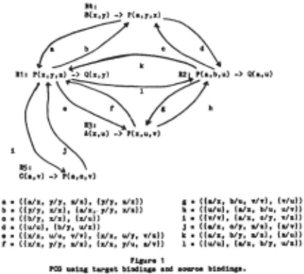
The match operation specifies a peg of a slightly different form. Instead of labelling the edge with the mgu, a directed edge linking a source node (S) to a target node (T) labelled with the target binding (~) and the source binding (4) is used. Figure 1 shows a peg consisting of five rules, labelled R1 through R5. While the rules considered in the remainder of this paper are of the form A & ··· & A -> C where j L 1 and all variables Are unive~sally quantifed (i.e. Horn clauses), SNIP is not so limited (see [19]). The edges are labelled with the pair (~,4) where ~ is the target binding and 4 is the source binding. The source node is the literal at the tail of the edge and the target node is at the head of the edge. For example, the edge labelled "a" in Figure 1 has P(a,y,x) as the source literal and P(x,y,z) as the target literal. SNIP does not explicitly store the peg but uses the match function described above to compute the edges on demand. The remainder of this paper is concerned with peg's of this last form.
3. Active Conoection Graphs
An actiye connection araph (acg) is a connection graph in which edges link literals and are labelled with a target binding and source binding. These graphs are active because instances of literals flow from one formula to another formula via the edges. Using the producer-consumer
analogy, a rule instance can be considered a producer of instances of its consequents and a consumer of instances of its antecedents. Furthermore, the acg contains instances of the rules in the peg, the edges in the acg point in the opposite direction to the corresponding edges in the peg and the bindings play an active role (see below). The target binding filters the flow of instances of literals. The source binding translates between variable contexts.
Suppose a consequent reasoning system has been asked to deduce all instances of Q using the peg of Figure 1. It can use R1 and R2 to deduce instances of Q if appropriate instances of P can be deduced. Thus, rules R3-R5 can be used. A full acg for this scenario is presented in Figure 2. Rectangles enclose formulas. The partitions contain literals instances. Antecedents appear on the left of the double line, consequents to the right. The rectangle at the top of Figure 2 represents the request to deduce all instances of Q and as such has an empty consequent part. In this example, each acg rule labelled Ai is an instance of the peg rule labelled Ri. These labels are arbitrary and the reader shOuld not infer anything about the construction of the acg based on the labels alone. The remainder of this section expands this simple notion of active connection graphs using the acg of Figure 2 as an example.
Target bindings and source bindings operate on the bindings flowing through the acg. A target binding is a ~ which only lets through those bindings which have the binding of the filter as a subset. For example, in the active connection graph of Figure 2, if G2 produced the bindings {alx, b/y, c/z} and {a/x, d/y, e/z}, only {a/x, b/y, c/z} would be allowed to pass through the filter <alx, bly> to A2. The source binding is used to ~ variable contexts. A2 contains only the variable u while G2 produces bindings with the variables x, y and z, so in order for G2 to send bindings to A2, the variable z must be mapped to the variable u. Continuing with the example above, since the binding {a!x, b/y, c/z} passed through the filter it next encounters the switch [z/u]. The switch uses the binding application operation defined in Section 2 to generate a new binding. In this case, {z/u} \ {a!x, b/y, c/z} yields {c/u}, which is an appropriate binding in the context of A2.
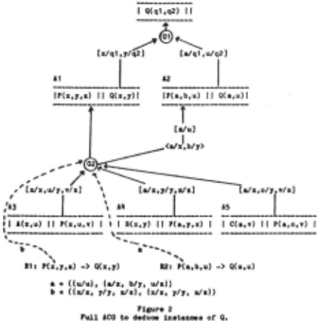
To deduce all instances of Q requires back c:haining through the peg until only ground literals are found or all possible rules are tried. Initially, a request is created which contains a literal . In Figure 2, Q(q1,q2) is that request. The next step is to create a &oal node for the literal. The goal node matches its literal with the peg to find all literals which unify with it. If there are ground instances then the source bindings of those matches are answers and the goal node produces them immediately. Other matches can be literals which are antecedents or consequents of rules in the peg. For every literal in the consequent of some rule, a new rule instance is added to the acg using the target bindings, and the instance is connected through a switch containing the source binding to the goal node. The same process of creating goal nodes is applied to each of the antecedents of the new rule instances created in the previous step. This process is repeated until either no more rules apply or only ground instances are found. However, a new goal node need not be created if an existing one will suffice. The remainder of this section describes how to find adequate extant goal nodes without doing extra matching and how to use results previously generated by a goal node.
Suppose a goal node is about to be created for some literal in a rule instance of an acg. Which other literals are likely to have goal nodes which should be checked? Namely, those other literals in the peg unifiable with the literal which are in the antecedent of some rule of the peg and which have already had goal nodes . created for them. Thus, when a new goal node performs its match as described above, the matched antecedent literals are marked with a pointer to the newly created goal node. These pointers, which link antecedent peg literals to goal nodes in the acg, are called &QAl pointers. Just like peg edges, each goal pointer is marked with a target binding and source binding. When a new goal node is about to be created, if its literal has no goal pointer then no existing goal node will be useful. If it does, it is possible that one of the goal nodes pointed to could be used instead of the proposed goal node.
Let's consider as an example the process of building the acg of Figure 2 using the peg of Figure 1. Recall that the request was for all instances of Q. A goal node is created for Q(q1,q2) and a match performed. The results of the match of Q(q1,q2) are the tuples <Q(a,u), {u/u}, {alq1, u/q2}> and <Q(x,y), {x/x,y/y}, {x/q1, y/q2}> . Both Q(a,u) and Q(x,y) are consequents of rules, so rule instances are created for them in the acg connected through the appropriate switches to G1. There are no goal pointers created because Q(q1,q2) does not match any literal in an antecedent of a rule. Continuing to expand the acg using the antecedents of A1 and A2 requires picking one of them to expand first. Whichever order is picked, the same acg is constructed.
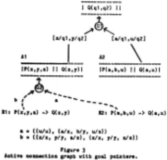
Suppose A1 is picked for expansion. First, the literal P(x,y,z) is checked for a goal pointer. There are none, so a new goal node is built for P(x,y,z). The result of the match are the tuples <P(a,b,u), {u/u}, {a!x, b/y, u/z}>, <P(x,u,v), {x/x, u/u, v/v}, {xlx, uly, v/z}>, <P(a,y,x), {y/y, x/x}, {a/x, y/y, x/z}>, <P(a,c,v), {v/v}, {a!x, ely, v/z}> and <P(x,y,z) 1 {x/x, y/y, z/z}, {x/x, y/y, z/z}>. P(a,b,u) is an antecedent of R2, so P(a,b,u) gets a goal pointer to the goal node for P(x,y,z). Also, P(x,y,z) is given a goal pointer to its own goal node. We draw a goal pointer as a dashed line labelled with the target binding and source binding of the match. Figure 3 shows the acg and part of the peg with goal pointers after this step. The remaining target literals are each consequents of some rule and the rules are added to the acg as before. Next, a goal node is to be created for P(a,b,u) of A2. But the peg literal P(a,b,u) in R2 has a goal pointer. Thus, some instance of the old goal literal, P(x,y,z), unifies with the literal which nas the goal pointer but the binding of the current acg rule instance is not necessarily compatible with the binding of the old goal literal.
In· the current example, the old target binding from the goal pointer is identical to the binding associated with A2. However, G2 is not identical to the proposed goal for P(a,b,u). Rule instance A2 is interested in a subset of all instances of P(x,y,z), namely those instances which have a/x and b/y, It is important to note that G2 will produce all that the proposed goal node for P(a,b,u) would produce and more. Also, above G2 all instances are in terms of the variables of R1. Instead of creating a new goal node for P(a,b,u) and the edges associated with it, G2 is reused. The results from G2 must be filtered by <alx, b/y> and variable contexts switched by [z/u]. The filter is computed from the application of the current binding to the old source binding. This assures that the filter contains variables which the old goal node produces. The switch is obtained by considering the binding pairs of the old source binding for which the term is a variable as a "variable map". Discarding those binding pairs for which the term is a constant and inverting the remaining pairs yields the appropriate binding for the switch. For example, discarding pairs with constant terms and then inverting {a!x, b/y, u/z} yields {z/u}. Figure 2 shows the acg after the filter and switch have been built.
If A2 were expanded before A1 then a goal node would have been created for it and goal pointers established from the antecedents of R1 and R2 to the goal node. To obtain the same acg requires that the goal node created for P(a,b,u) in A2 be superseded by the goal node eventually created for P(x,y,z). When a goal node is superseded, it is erased from the acg and all the consumers of the superseded goal nodes become consumers of the new, more general goal node with an appropriate filter and switch between the superseding node and the old consumers.
We stated above that rule instances in the acg consume instances of antecedents and produce instances of consequents but have totally ignored what constitutes such an instance. There are basically two alternatives. An instance of a literal can be either a separate literal or a reference to a literal and a binding which when applied to the literal would yield an instance of it. We prefer the second alternative because the inference algorithms need not produce extra literals and because the match operation mentioned above returns such information. Furthermore, information about literals is superfluous in communication between rule instances in the acg because the literals are known to unify (that's why there is an edge in the peg) and therefore, only bindings need be communicated along the edges of the active connection graph.
Finally, we mentioned above that the acg contains rule instances but the previous examples use the peg rules directly. In general, rule instances in the acg are pairs -- a rule from the peg and an associated binding. The rule instances in the examples all have an identity binding, i.e. a binding in which each variable of a binding pair is bound to itself. The binding is used to restrict the rule instances to generating just those literal instances which are requested. In other words, it is used as an internal filter in the rule instances in order to keep the inference more focussed.
In summary, an acg contains instances of rules which are linked to each other through filters, switches and goal nodes. The separation of the target and source bindings allow rule instances to work in their own variable environment, relying on the source binding of the peg to enable switching of variable contexts and on the target bindings to allow more general producers to be used by less general consumers. The goal nodes are the production site of instances of literals and so are useful to more than one consumer. Finally, goal nodes are indexed on antecedent literals using goal pointers.
4.Recursiye rules cause cycles
A set of recursive rules is of the form A & ··· &A -> B , B & ··· & Bk -> ... -> C, with C unifiabie wit~ at least one of the antecedents, A 1 say. In an acg, this means that the goal node for C can be used instead of creating a new goal node for A · As an example, consider the peg of Figure 4 whi~h contains the recursive ANCESTOR rule. The two rules represent the predicate calculus statements V(x,y,z)(ANCESTOR(x,y) & ANCESTOR(y,z) -> ANCESTOR(x,z)] and V(x,y)(PARENT(x,y) -> ANCESTOR(x,y)]. The remainder of the entries represent the ground literals PARENT(Bill, John), PARENT(John, Mary), ANCESTOR(Bill, Bob), ANCESTOR(John, Mary) and ANCESTOR(Mary, Sarah). Since the ground literals are never a source node in a match, the edges from the ground literals to literals in rules are omitted.
Consider a request, ANCESTOR(q1,q2), for all instances of the ANCESTOR relation. Inference proceeds by creating a goal node for the request, creating rule instances for all rules in the peg which have the literal as a consequent and creating a goal pointer for each literal in the antecedent of some rule. Figure 5 shows the acg at this point. Here, instances which are produced are shown in terms of the variables of the goal literal next to the goal nodes which collect them. When such an instance is produced, it flows through the acg until either it encounters the top level request or it is consumed by a goal node which has previously produced it. Thus, the bindings {Bill/q1, Bob/q2}, {John/q1, Mary/q2} and {Mary/q1, Sarah/q2}, representing the ground literals ANCESTOR(Bill, Bob), ANCESTOR(John, Mary) and ANCESTOR(Mary, Sarah) respectively, are stored by G1 and consumed by the top level request. Picking one rule instance, A1 or A2, to expand first has no significant impact because if A2 were expanded first then any results derived from A2 would be stored in the goal node just as these are. The order of the creation of the goal nodes in A1 is insignificant for this example because both reuse G1.
| a • ((ols,olsl, (o/x,o/rll | 1 • {{), {1111/s,Bob/J)) |
| t. • ((alx,r/r), {alx,r/a)) | J. {{), {Joho.ts,Marr/rll |
| a • ((o/s,o/sl, {o/J,o/sl) | t. {{), {Harr/x,Sarablrll |
| • • ({r/r,vsl, lr/s,oJ•ll | 1. ({), {Marr/r,Sarablsll |
| a • ({ols,rtrl, {olx,rtrll | • • ((J, {Jolu>/r,Marrtsll |
| t • ( (ols,rtrl, {o/x,rtrl l | a • {{), {8111/J,Bob/s)) |
| • ((J/J,o/s), {J/&,&/Jll | o • {{), {8111/x,Jobo./J)) |
| I a • ({o/s,rtrl, {&/J,r/sll | p • ({), {Joho.ts,Marr/rll |
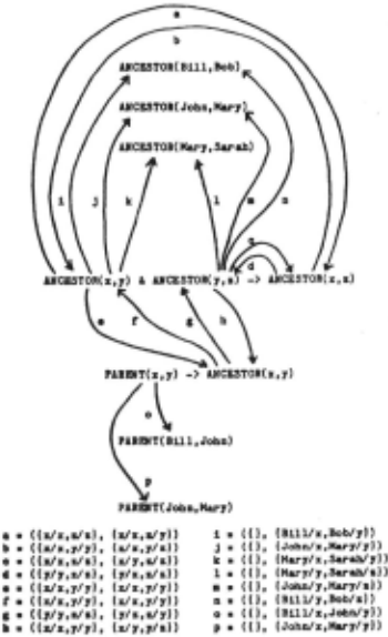
Consider ANCESTOR(x,y) as the first goal literal. ANCESTOR(x,y) has the goal pointer ({x/x, y/y}, {x/q1, y/q2}), and the binding associated with it in A1 is {x/x, y/y}. Thus, the goal pointer's old target binding is identical to the rule instance binding and G1 can be used. This is accomplished by giving G1 another consumer, the ANCESTOR(x,y) antecedent, connected through the switch [q1/x, q2/y]. The bindings from G1 are produced for this new consumer but further processing by A1 is not possible because the other antecedent of A1 has not yet consumed any instances of ANCESTOR(y,z).
Goal nodes act as data collectors [13, 19]. A data collector stores all literals it has consumed and never produces a literal it has previously produced. When an old goal node is given an additional consumer, all literals previously produced are immediately available to the new consumer. Also, the new consumer receives any new literals produced by the goal node. The fact that data collectors never produce the same literal twice protects SNIP from getting into an infinite loop by prohibiting the passing of the same literal around a cycle in the acg.
Next, consider trying to create a goal node for ANCESTOR(y,z). Again, G1 is found using the goal pointer and as before the old target binding and the binding of the rule instance are identical.
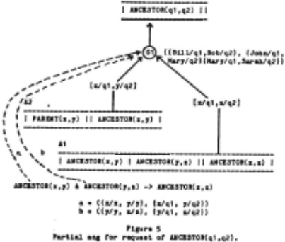
A new consumer is added to G1 through a switch of [y/q1, z/q2] and the three instances stored by G1 are produced for this new consumer. Since A1 has now received the bindings {Johnlx, Mary/y} for one antecedent and and {Mary/y, Sarah/z} for the other, it can produce {Johnlx, Sarah/z} and pass it to G1. Again, G1 produces {John/q1, Sarah/q2} to all consumers because it has not produced it before. Now, A1 cannot produce any further instances.
Finally, a goal node is created for PARENT(x,y), call it G2. Since there are no goal pointers for PARENT(x,y), a match is performed resulting in the ground instances of {Bill/x, John/y} and {John/x, Mary/y}. Figure 6 shows the acg after G2 has matched these instances. These are stored by G2 and produced to all consumers. A2 now has its antecedent satisfied in the bindings above. Since these instances are next passed to G1 and {Bill/q1, John/q2} has not been produced before, it is produced to the top level request and the other consumers. After passing through the switches, the appropriate binding arrives in A1 which produces ANCESTOR(Bill, Mary). Again, G1 has not produced {Bill/q1, Mary/q2} previously, so it passes it on to all consumers. A1 in turn produces {Bill/x, Sarah/z} to G1. Since G1 has not previously produced {Bill/q1, Sarah/q2}, it produces this binding to all consumers. Now, no further results can be produced by A1 and since there are no other rules left to expand, inference terminates.
This example demonstrates that recursive rules can be productively used in an acg and not cause an infinite loop. The reason no infinite loop is encountered is that no further results could be produced and that the acg contains a cycle as opposed to continually trying to use the recursive ANCESTOR rule. This example also demonstrates the accessing of data stored by a goal node previous to adding a new consumer. This is a property of the goal node acting as a data collector. Finally, this example suggests how rule instances produce bindings, waiting until sufficient instances have been consumed in the appropriate binding. SNIP
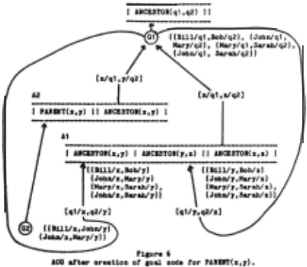
allows other logical connectives so that other schemes for rule instances to produce instances of their consequents are required (see [18]). Note, this kind of structure is built for indirectly recursive rules as well as the directly recursive rule in the above example, the resulting active connection graph is a directed &raph and neither a tree nor a directed acyclic graph, and once it is built its size is constant.
5.Summary
In SNIP, recursive rules cause cycles to be built in an active connection graph. The key features of active connection graphs which allow recursive rules to be handled are: 1) goal nodes are data collectors; 2) data collectors never produce the same answer more than once; 3) the data collector may report to more than one consumer; 4) a new consumer may be assigned to a data collector at any time -- it will immediately be given all previously collected data; 5) variable contexts are localized, switches change contexts dynamically as data flows around the graph; 6) filters allow more general producers to be used by less general consumers; 7) goal nodes are indexed on antecedent literals which were matched by the goal literal.
@inproceedings{ijcai1981p72,
  title     = {Using Active Connection Graphs for Reasoning with Recursive Rules},
  author    = {McKay, Donald P. and Shapiro, Stuart C.},
  booktitle = {Proceedings of the Seventh International Joint Conference on
               Artificial Intelligence, {IJCAI-81}},
  publisher = {International Joint Conferences on Artificial Intelligence},
  editor    = {Patrick J. Hayes},
  pages     = {368--373},
  year      = {1981},
  month     = {8},
  note      = {INFERENCE and REASONING},
  url       = {https://ijcai.org/proceedings/1981/72},
}
TY - CPAPER TI - Using Active Connection Graphs for Reasoning with Recursive Rules AU - McKay, Donald P. AU - Shapiro, Stuart C. T2 - Proceedings of the Seventh International Joint Conference on Artificial Intelligence, IJCAI-81 PB - International Joint Conferences on Artificial Intelligence PY - 1981 SP - 368 EP - 373 UR - https://ijcai.org/proceedings/1981/72 ER -Copied
Machine-readable versions of this paper, for tools and AI agents:





