
Parameter Networks: Towards a Theory of Low-Level Vision
Proceedings of the Seventh International Joint Conference on Artificial Intelligence. Invited Talk. Pages 1068-1077.
© 1981 International Joint Conferences on Artificial Intelligence
Abstract
One of the most fundamental problems in vision is segmentation; the way in which parts of an image are perceived as a meaningful whole . Recent work has shown how to calculate images of physical parameters from raw intensity data. Such images are known as intrinsic images, and examples are images of velocity (optical flow), surface orientation, occluding contour, and disparity. While intrinsic images are not segmented, they are distinctly easier to segment than the original intensity image. Segments can be detected by a general Hough transform technique. Networks of feature parameters are appended to the intrinsic image organization. Then the intrinsic image points are mapped into these networks. This mapping will be many-to-one onto parameter values that represent segments. This basic method is extended into a general representation and control technique with the addition of three main ideas: abstraction levels; sequential search; and tight counling. These ideas are a nucleus of a connectionist theorv of low - '•~ve~ and intermediate-level vision . This theory explains segmentation in terms of massively parallel cooperative computation among intrinsic images and a set of parameter spaces at different levels of abstraction. The preparation of this paper was supported in part by the Defense Advanced Research Projects Agency, monitored by the ONR, under Contracts N00014-78-C0164 & N00014-80-C-0197.
- Aallard, D.H., "Generalizing the Hough transform to detect arbitrary shapes," TR55, Computer Science Dept, U. Rochester, October 1979; l'allern Recognition 13, 2, 111-122, 1981 a.
- Ballard, D.H ., "Shape and illumination angle from shading," Computer Science Dept, U. Rochester, 198lh.
- Ballard, D.H., "3-d rigid body motion from optical flow," Computer Science Dept, U. Rochester, 1981c.
- Ballard, D.H . and C.M . Brown . Computer Vision. Prentice Hall, in press, to be released February 1982.
- Ballard, D.H. and D. Sabbah, "On Shapes," 7th IJCAI, Vancouver, A.C., Canada, 1981.
- Barnard, S.'r. and W .B. Thompson, "Disparity analysis of images," TR 79-1, Computer Science Dept, U. Minnesota, January 1979.
- Barrow, H.G. and J.M. Tenenbaum, "Recovering intrinsic scene characteristics from images," TN 157, AI Center, SRI lnt'l, April 19n.
- Brandt, A., "Multi•level adaptive solutions to boundary• value problems," Math ofComp 31, 138, 333•390, April 1977.
- Bribiesca, E. and A. Guzman, "How to describe pure form and how to measure differences in shapes using shape numbers," Proc., IEEE Computer Society Conf on Pattern Recognition and Image Processing, 427•436, Chicago, IL, August 1979.
- Bruss, A.R., "The image irradiance equation: its solution and application" (Ph .D. thesis), TR 623, AI Lab, MIT, 1981.
- Duda, ItO. and P.E. Hart, "Use of the Hough transform to detect lines and curves in pictures," CACM I 5, 1, 11•15, January 1972.
- Feldman, J.A. and D.H. Ballard, "Computing with connections," TR72, Computer Science Dept, U. Rochester, 1981.
- Fischler, M.A. and P. Rarrett, "An iconic transform for sketch completion and shape abstraction," Computer GraphicJ Image Processing 13, 334•360, 1980.
- Hanson, A.R. and E.M. Riseman, "Segmentation of natural scenes." in A.R. Hanson and E.M. Riseman (Eds). Complller Vision Systems. NY: Academic Press, 1978.
- Hinton, G.E, "Relaxation and its role in vision," Ph.D. dissertation, U. Edinburgh, 1979.
- Horn, B.K.P and B.G. Schunck, "Determining optical flow," AI Memo 572, AI Lab, MIT, April 1980.
- Horn, B.K.P. and R.W . Sjoberg, "Calculating the reflectance map," Proc., DARPA IU Workshop, liS• 126, Pittsburgh, PA, November 1978.
- Hough, P.V.C., "Method and means for recognizing complex patterns," U.S. Patent 3,069,654, 1962.
- Hummel, R. and S. Zucker, "On the foundations of relaxation laheling processes." TR, Dept. of Electrical Engineering, McGill U., 1980.
- Hurvich, L.M. and D. Jameson, "An opponent-process theory of color vision," Psych Review 64, 384•390, 1957.
- Ikeuchi, K., "Numerical shape from shading and occluding contours in a single view," AI Memo 566, AI Lab, MIT, revised February 1980.
- Kanade, T., "Recovery of the three-dimensional shape of an object from a single view," CMU•CS-79•153, Computer Science Dept, Carnegie-Mellon U., October 1979.
- Kanade, T., "A theory of Origami world," CMU•CS-78• 144, Computer Science Dept, Carnegie-Mellon U., 1978.
- Kender, J.R., "Shape from texture: A brief overview and a new aggregation transform," Proc.. DARPA IU Workshop, 79•84, Pittsburgh, PA, November 1978.
- Kender, J.R. and T. Kanade, "Mapping image properties into shape constraints: Skewed symmetry, affine• transformable patterns, and the shape•from•texture paradigm," Proc., .lst Annual Nat'l. Conf. on Artificial Intelligence, 4•6, Stanford U., August 1980. 1078
- Kimme, C., D.H. Ballard, and J. Sklansky, "Finding circles by an array of acccumulators," CACM 18, 1, 120•122, February 1975.
- Lawton, D.T., "Constraint-based inference from image motion," Proc., 1st Nat' I. Con f. on Artificial Intelligence, 31•34, Stanford U., August 1980.
- Marr, D., "Representing visual information," in A.R. Hanson and E.M. Riseman (Eds). Computer Vision SyJtems. NY : Academic Press, 1978.
- Marr, D., "Representing and computing visual information," in P.H . Winston and R.H. Brown (Eds). Art(ficia/ Intelligence: An MIT Perspective. Cambridge, MA: The MIT Press, 1979.
- Marr, D. and T. Poggio, "Cooperative computation of stereo disparity," Science 194, 283• 287, 1976.
- Ohlander, R., K. Price, and D.R. Reddy, "Picture segmentation using a recursive region splitting method," CGIP 8, 3, December 1979.
- Prager, J .M., "Extracting and labeling boundary segments in natural scenes," JFn:• Trans. PAM/ 2, 1, 16•27, January 1980.
- Rosenfeld, A., R.A . Hummel, and S.W. Zucker, "Scene l:dlL•IIil!t' l>v rt•l:lx:tlltt ll "JII.'I':tli""~'-" /1-.FF 'J'mm. Sflff • I• J'Jf(, Sabbah, D., "Design ol a highly parallel visual recognition system," 7th IJCAI, Vancouver, B.C., Canada, 1981.
- Shapiro, S.D., "Generalization of the Hough transform for curve detection in noisy digital images," Proc., 4th IJCPR, Kyoto, Japan, 710• 714, November 1978.
- Sloan, K.R., Jr., "Dynamically quantized pyramids," 7th IJCAI, Vancouver, B.C., Canada, 1981. IJCAI
- Tanimoto, S. and T. Pavlidis, "A hierarchical data structure for picture processing," CGIP 4, 2, 104•119, June 1975.
- Ullman, S., "Interpretation of visual motion," Ph.D. dissertation, MIT, 1977.
- Ullman, S., "Relaxation and constrained optimization by local processes," CGI P 10, 115•125, 1979.
- Zucker, S.W., "Labeling lines and links: An experiment in cooperative computation," TR 80•5, Computer Vision and Graphics Lab., McGill U., February 1980 ..
- Zucker, S.W., "Relaxation labelling and the reduction of local ambiguities," TR 451, Computer Science Dept, U. Maryland, 1976.
References were extracted automatically from the PDF and may contain errors.
Full text extracted automatically from the PDF; figures, tables and equations may differ. The PDF is the version of record.
1. Overview
One of the most troublesome puzzles in vision is how parts of an image are seen as a meaningful whole or segment. This is known as the segmentation problem. The ambiguous use of segment, which means part, to denote a whole, arises from the fact that a segment is an intermediate component in a description which relates an object with an image. From the viewpoint of the object description, the segment is a part. From the viewpoint of a group of image points with common properties, the segment is a whole.
Parts of an image are seen as a segment if the corresponding physical object has common physical or geometric properties, or features. For example, if a connected component of the image has a single color, say red, then it may be seen as a segment. The patch of red arises from the physical object's surface reflectance. Usually there are not one but several features which have the same Many factors make segmentation difficult. For example, features are not always spatially registered. Given a multicolored cube, which feature should be the most compelling, the color or the geometric lines indicating the cube? In the general case this answer depends on the goals of the perceiver. Another common problem occurs when an object is occluded; a theory of low-level vision must be able to explain how an object is seen as a segment when the features are only partially registered or incomplete. Real image data is also noisy and many segments are only perceived owing to the combination of weak evidence of several features. The evidence may be so weak that each feature, if viewed in isolation, would be uninterpretable.
Evidence from psychology suggests that the minimum time for human beings to respond to a visual stimulus is approximately JOO ms. If the time constant for a neural unit is approximately 2 ms, this means that about 50 cycles are available for the complete perceptual processing and motor response in thi~ case. The human brain has about 1011 neurons, any of which may be involved in the processing. If connections must go through intermediate units, the best strategies involve on the order of the logarithm of the number of neurons. Thus there is little time to do more than link up the right neurons. Arguments like these support connectionist theories of brain processing:
"The connectionist view of brain and behavior is that all encodings of importance in the brain are in terms of the relative strengths of synaptic connections. The fundamental premise of connectionism is that individual neurons do not transmit large amounts of symbolic information. Instead they compute by being appropriately connected to large numbers of similar units." [Feldman and Ballard, 1981]
We develop the nucleus of a connectionist theory of low-level and intermediate-level vision which explains the above aspects of segmentation in terms of massive/~ parallel cooperative computation [Rosenfeld et al., 1976; Zucker, 1976; Marr, 1979] between two groups of networks. One group, intrinsic images (Barrow and Tenenbaum, 1 978], can be computed primarily in terms of local constraints. The other, termed a feature space, can be computed primarily in terms of global mappings from intrinsic images to feature space. Feature space is also distinguished from intrinsic image space in that it is not retinotopic. f-eature space itself may have many different levels of abstraction.
Intrinsic images and feature spaces are collectively called parameter networks because they both have a common organization. That is, the network is an organization of basic units, each representing a value of a particular parameter. The basic element of a parameter network is a parameter unit. A parameter unit will represent a single parameter value and has an associated confidence. The value is a set of numerical measurements for the node; the confidence is a measure of their believability. For example, if there is an edge at (10,10) with orientation 30· and length 5 units, the ve~.:tor value of the parameter node representing the edge is {x,y,O,s) = {l0,l0,30·.s). The associated confidence is a measure of the fuzziness of this estimate. One way a confidence may be increased is if there are nearby edges of the same orientation which align. Thus in Figure 1 the edges in (a) and {b) have the same value but we can be more confident in case (b).

Collections of value units form networks. Each value unit is connected to a subset of other value units, and can alter only the confidence of those units. Underlying physical principles determine the appropriate connection subsets. The confidence updating is done by non-linear relaxation. In this formalism, a segment has a simple interpretation: it is a set of high-confidence units which are connected. The overall structure of the paper shows how abstractions of physical principles lead to connections in networks. The reader interested in more implementation details should consult [Feldman and Ballard, 1981]. The principal elements of the theory are the following.
- A lowest level of abstraction consisting of several intrinsic images which are computed simultaneously.
Recent work has shown how to calculate intrinsic images from intensity data. Examples are images of velocity (optical flow) [Horn and Schunck, 1980; Ullman, 1977; 1979), surface orientation [Horn and Sjoberg, 1978; Ikeuchi, 1980], occluding contour [Prager, 1980; Rosenfeld et al., 1976], and disparity [Marr and Poggio, 1976; Barnard and Thompson, 1979]. Intrinsic images can be computed independently under special conditions, but in general they are interdependent. Intrinsic images are in concert with the hypothesis that the visual system builds many intermediate descriptions from image data. These descriptions represent important parameters such as velocity, depth, surface reflectance explicitly, since in the explicit form they are easier to map into object descriptions.
- Intermediate levels of abstraction consisting of feature spaces.
If parts of the intrinsic image are organized in some way, this organization can be detected by a general Hough transform technique [Duda and Hart, 1972; Ballard, 19H1a; Kender, 1978; Ohlander et al., 1979] termed a constraint transform. This is done by describing the organization in terms of more abstract parameters and then mapping the intrinsic image points into parameter space. The transformation will be many-to-one onto parameter values which represent meaningful segments. Major advantages of the Hough transform are that it is relatively insensitive to occlusion and noise.
3) Hierarchies involving several levels of abstraction.
The constraint transform is a way of seeing spatial information as a unit. However, if the unit has a complex structure the mapping from space to unit can be unmanageably complex. A way around this is to introduce units at several levels of abstraction [Sabbah, 1981; Ballard and Sabbah, 1981; Kender, 1978]. This reduces a complex transform to several simpler transforms between units at successively higher levels of abstraction.
4) Focus-ofattention mechanisms.
Vi~·ual focus-of-attention can be partly explained as the conjunction of two mechanisms: I) the use of constraint transforms to modify sensor input; and 2) the seqllrntial application of constraint transforms.
- Coupling between intrinsic images and feature spaces. In general, intrinsic images cannot be computed without global parameters. At the same time, these global parameters are what we mean by seeing parts of the intrinsic image as a segment. In these cases the intrinsic image and parameters are said to be tightly coupled; although each cannot be computed independently, they can be computed simultaneously [Ballard, 1981 b; 1981c].
We re-emphasize that our interest is low-level vision. Thus in item (4) above, focus of attention is interpreted in a narrow sense: visual features which are clear can help the recognition of other features (or perhaps direct eye movements). We do not attempt to explain general plans and goals.
2. Intrinsic Images
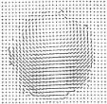
An intrinsic image is an image of some important parameter that is in registration with the original intensity image [Barrow and Tenenbaum, 1978; Marr, 1979], that is, each parameter is indexed by retinal coordinates. For example, in the velocity (optical flow) image, one is able to compute at each point in time and for each spatial position a local velocity vector v{x,t). Figure 2 shows Horn's example for a rotating sphere [Horn and Schunck, 1980]. Intrinsic images may only be computable over certain parts of the image, and over those parts the parameters are continuously varying. While intrinsic images are not segmented into parts of objects, they are distinctly easier to segment than the original intensity image.
··························
Somewhat surprisingly, intrinsic images can all be computed in a similar manner. Two constraints, one derived from r>hysical prirH.:;ples and the other from a constraint that Ure resultant images should be locally smooth, suffice to specify a parallel-iterative algorithm. Table 1 shows this commonality but is not an exhaustive list of approaches.
| Parameter | Physical Constraint | Smoothness Constraint |
| Edge Orientation /) | boundaries are locally linear | nearby edges should align [Prager, 1979] |
| Disparity d | if x corresponds to x · then f(x + t.)= f(x · + t.) | neighboring points should have similar disparities [Marr & Poggio, 1976] |
| Surface | f(x) = R(o ,<p,fls·'l's) | v2o=O |
| Orientation (} ,q> | Ds·'Ps is the light source direction | v2'1' =0 [lkeuchi, 1980] |
| Optical Flow U,V | df/dt=O | v2u=O v2v=O [Horn & Schunck, 1980] |
While the above algorithms work well on images which are constrained to satisfy the underlying assumptions, they may not work in the general case. Almost always there are free parameters or boundary conditions which have to be determineu independently. For example, in the surface orientation, a boundary contour is necessary [Bruss, 1981].
2.1 Multi-Resolution l~elaxation Methods
One notion of "boundary condition" is image resolution. Previous methods for computing intrinsic images have used a single image resolution, but in most situations this is unrealistic. What is the correct resolution? At high resolution: (1) noise is a factor; (2) convergence is slow; and (3) basic assumptions may not hold. To see the last point, imagine trying to compute shape from shading using a surface with a micro-texture. At low resolution the surface structure is blurred and simple reflectance models hold, but at high resolution the microstructure can render such models useless. I .tJw resolution may not always be appropriate, however. Even though noise is less of a factor and convergence is fast, basic assumptions may still not hold. The last point arises from the fact that most intrinsic images are computed from constraints which assume local variations are smooth. With increasing grid resolutions, these assumptions are less likely to be valid.
Hence a conjecture is that there is a range of resolutions for which the computations will be valid. Furthermore, this range is expected to be spatially variant. A tool for exploring this conjecture is multigrid relaxation techniques
[Brandt, 1977], which have proven very useful for solving differential equations. This model, together with reasoning from physical first principles, should allow tht: dt:termination of image-dependent grid resolutions for which intrinsic image computations are · valiu. Multigrid techniques are of course related to pyramids [Tanimoto and Pavlidis, 1975; Hanson and Riseman, 1978; Sloan, 1981].
2.2 Cooperative Computation of Multiple Intrinsic Ima~-:es
Intrinsic images are logically computed simultaneously. In fact, they have to be; otherwise each intrinsic image is underdetermined in the general case. (Only on certain synthetic images is the computation well-defined.) Furthermore, they are highly interdependent, particularly at points of discontinuity [Barrow and Tenenbaum, J 978]. For example:
- intensity edges can be indicative of depth discontinuities. Thus the edge image is coupled to the disparity image;
- surface orientation is also indicative of depth discontinuity and is thus related to the other two; and
- different objects ·which are moving relative to each other produce discontinuities in the flow field.
By incorporating these couplings in the intrinsic image computations, one should find general cases where the computations will converge. A separate issue is the behavior of the coupled computations in the face of conflicting information.
2.3 Intrinsic Images at Different Levels of Abstraction
The survey of intrinsic images (Table 1) excluded the fact that intrinsic images may have line structure involving several levels of abstraction. In fact, it seems likely that multiple abstraction levels are necessary in many .cases. For example, Zucker [1980] uses two levels of abstraction in computing orientation intrinsic images, one for points of high gradients and the other for edge segments. The computation of a velocity image in 3-d could involve three:_ levels of abstraction:
- a change detection level where units are used for variations in intensity over space and time 6fl6x ·, Bf!By ·, Bfl Bt (primes denote retinal coordinates);
- an optical flow level where units correspond to retinal velocities (u(x · ,y · ),v{x · ,y · ));
- a 3-d flow level where units correspond to 3-d velocities (v x{x,y ,z), vy{x,y,z), v 2 {x,y ,z)).
The feasibility of computing the optical flow from change measures has been studied by [Barnard and Thompson, 1979; Prager, 1980; Horn and Schunck, 1980]. The feasibility of computing 3-d flow is explored in [Ballard, 198lc].
2.4 Intrinsic Images and Parameter Nodes
Two models have been used to compute intrinsic images: 1) the value unit defined in Section J [Prager, 1980;
Marr and Poggio, 1976]; and 2) a variable unit [lkeuchl, 1980; Horn and Schunck, 1980]. In the first model there is a unit for every value of every variable; in effect the representation has only constants. Constant value units may have outputs which are confidences between zero and one. In the second model, each unit represents a variable which can take on values {the standard method is to use an array for these units). The output is the value; there is no explicit notion of confidence.
In general the unit/value representation is sufficient since problems formulated to use variables can be transformed into unit/value problems in the following manner. Suppose x, y, and z satisfy a relation R(x,y,z) = 0. Let us use a set of values A for x, 13 for y, and C for z. Where a E A, we would like C(a) to be 1 if there exist b E R and c E C such that C{b) = 1, C(c) = 1, and R{a,b,c) = 0. To implement this in a parameter network connect all pairs of (b,c) E BxC to a value (a) if R{a,b,c) = 0. Then starting with initial confidences, increment C(a) if there exist {b,c) such that R{a,b,c) = 0 and C(b) + C(c) > some threshold. The individual values b and c may be treated similarly.
Note that the updating function is nonlinear, when the underlying physical relation R is nonlinear. If the relation R can be linearized then the cooperative computations can be shown to be equivalent to linear programming [Hinton, l 979]. The linear case has also been analyzed by [Hummel and Zucker, 1980].
3. Feature Spaces
What does it mean to perceive parts of an image as a segment? In our theory, this perception takes place if there is a feature space such that each of the parts can have the same parameter value. This general idea is illustrated by the following examples.
- Parts of a color image may be seen as a segment if they have the same color. In this case the parameter space is a space of colors and the parts map into a common point representing the common color.
- Parts of an optical flow image may be seen as a segment if they are part of a rigid body that is moving. In this case the parameter space represents the rigid body motion parameters of translational and rotational velocity and parts of the image map into a common point in that space.
- Parts of edge and surface orientation images may be seen as a segment if they are part of the same shape. This case is more complicated as there must exist some internal representation of the shape. Given this representation, the parameter · space represents the transformation (scale, rotation, translation) from the internal representation to the (viewer-centered) image representation. Parts of the image which are seen as the shape have common values for these parameters.
A general way of describing this relationship between parts of an image and the associated parameters is a connectionist interpretation of the Hough transform [Hough, 1962; Duda and Hart, 1972; Kimme et al., 1975; Shapiro, 1978] which we have termed constraint transforms. In our low-level vision theory, constraint transforms relate intrinsic image units to feature units at different levels of abstraction. If an intrinsic image parameter is a vector unit {x,a(x)) in an intrinsic image space A and an element of feature space is a vector b in a feature space B then there is usually a physical constraint that relates a(x) and b, i.e., some relation f{a,b) such that f{a,b) = 0. The general form of f{a,b) is a table since f may not have an analytic form.
The space A represents all possible intrinsic image values. A particular intrinsic image is described by a set of values I ak} where ak = a(xk). Now the set {ak} is only consistent with certain elements in the space 13, owing to the constraint imposed by the relation f. This physical constraint can be exploited in the following manner. For each ak compute the set
Bk is the set of nodes in the feature space network B that the ak unit must connect to. Define H(b) as the number of times the value b occurs in UkBk (the union of all sets Bk). H(b) is the constraint transform from the space ~ to the space b and is the number of points in intrinsic tmage space whtch are consistent with the parameter value b. H(b) ma~es the most sense when the values both (a(x),x) and b are dtscrete. Hence the constant 6b above is related to the quantization in the space R. H is also best normalized by defining C(b) : = H(b)/l:bH(b). In that case, the value C(b) can stand for the confidence that the segment with feature value b is present in the image. H(b) can be thought of as a htstogram and C(b) a normalized histogram.
Concerning the implementation of constraint transforms in networks, Bk c B is the subset of R units to which the unit ak hould be connected in the network. A separate Hmax unit· is needed for normalization.
. ~rh.e _constraint transform need not originate from tntrtnstc tmage space but can be defined between any two spaces A and B as long as there is some relation f{a,b) = 0 for a E A and b E B. To avoid describing the above computations in detail, we use a shorthand notation for constraint transforms. Each transform can be described as the ~~pie <a,b,f> where the necessary computations are tmphctt. Note that the order of a and b is important in the notation; in general, <a,b,f> is not equivalent to <b,a,f>.
As a very simple example of a constraint transform we describe how a patch of red in an image may be seen 'as a unit. For this to happen, an association is made between the spatially contiguous points in the image and the particular value "red" in a parameter space of colors. There are essentially three dimensions to color space. Although r-g-b is widely used in computer applications, humans seem to use an opponents-process basis (r-g, y-b, white-black) [Hurvich and Jameson, 1957]. Denote this transformation by T. Then the constraint transform is given by <a,b,f> where
a = (r(x,y), b(x,y), g(x,y))
b = (rg, yb, bw) and
f = Ta - b
Figure 3 shows this idea, which has been used by [Hanson and Riseman, 1978; Oblander et al., 1979], applied to a color image.
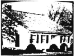
Figure 3: Segmentation in Color Space.[H:ln.SOI\ c:a~ RtstiiiAII],
The transformation results in a set of very sparsely distributed high-confidence feature space units. In our own work, color space is represented by rgb units in a threedimensional space of 163 total units. Only approximately 1% of the units have maximum confidence values. This figure is also typical of other modalities. In general, each ak and the relationship f will not determine a single unit in Bk but there still will be isolated high-confidence units. Figure 4 shows why this is the case: different ak units connect to common units in the feature space B.
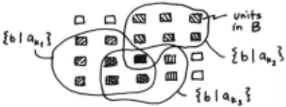
Figure 4
Of course segmentation must involve ways of associating peaks in several different feature spaces and methods for doing this are discussed in Section 6, but the cornerstone of the techniques are high-confidence units (histogram maxima) in the individual-modality feature spaces.
One might think that this is a cl\lstering technique presented with a different formalism. The constraint transform method is similar to clustering but differs in an important way. In general, feature space units are not independent but may interact through mutual connections. For example, consider L-joint units in an origami world feature space [Sabbah, 1981). Opposing L-joint units increase the confidence of each other. These kinds of effects are disallowed in clustering models.
Table 2 shows some other constraint transforms.
Table 2: Constraint Transforms
A: Intrinsic Image R: Feature Space
Color
Disparity
Optical Flow
Surface Orient'n.
- Segments of constant color [Ohlander et al., 1979; Hanson and Riseman, 1978)
- Surface orientation [Kender, 1978)
- Segments of constant disparity [Fischler and Barrett, 1980)
- Heading [Lawton, 1980; Prager, 1980) .
- Rotation of 3d rigid body [Ballard, 1981c]
- Illumination angle [Ballard, 1981b]
- Shape [Ballard and Sabbah, 1981)
- Occluding Contour · Shape [Kimme et al., 1975; Duda and Hart, 1972)
Texels
- Surface orientation [Kender and · Kanade, 1980)
To show how intrinsic 1mages and parameter spaces. may be related in more complicated ways, we briefly describe an example of how a specific two-dimensional shape is detected by specifying a constraint transformation from edge space (local linear edges detected with a standard edge detector) to a four-dimensional parameter space consisting of local origin coordinates, rotation and scale. Both the color-space example and this one have the same solution at an abstract level. In each case there is a transformation from intrinsic image space to parameter space that segments the image. In the first case, points in the color image have the same color values. In the second case, points in the edge image have the same shape parameter values.
3.1 Constraint Transforms: Two-Dimensional Sitapes
Known two-dimensional shapes can be located in a primal sketch [Marr, 1978] by encoding the shape information in a constraint table [Ballard, 1981a). The problem reduces to finding the parameters of the transformation from the viewed shape to its internal representation. Consider the case where an object being sought has no simple analytic form, but has a particular ~ilhouette. Suppose for the moment that the object appears m the image with known shape, orientation, and scale, so that its location is the only unknown parameter set. (If orientation and scale are unknown, they can be handled as additional parameters, as will be shown.) Now pick a coordinate system for the silhouette and draw a line to the boundary from the coordinate system origin. At the boundary point, compute the gradient direction and length and store the reference point as a function of this information. Thus it is possible to precompute the offset vector (r,a) of the reference point from boundary points given the gradient angle. The basic strategy of the constraint technique for shapes is to compute the loci of reference point units in parameter space from an edge In image space and raise the confidence of those units. In this case the reference point coordinates (xc,yc) are the only parameters (remember, rotation and scaling have been fixed). Thus an edge point (x,y) with gradient orientation (cp) and span (I) determines the possible reference points to be at
(x + r(cp,l}cos(a(cp,l)},y + r(cp,l)sin(a(cp,l))).
In tenns of our constraint transform notation. the transform is of the form
<( cp( x,y ),1( x,y },x,y ).( xc,yc}, T>
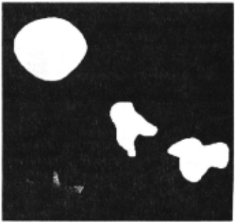
where Tis the constraint relation between (cp(x,y),l(x,y},x,y) and (xc,yc). The results of using this transform to detect a shape are shown in Figures S and 6. Figure S shows an image of shapes. The constraint table was made for the middle shape. Figure 6 shows the constraint Transform for the shape, i.e., H(xc,yc) displayed as an image.
Figure S
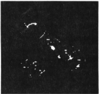
What about the parameters of scale and rotation, s and fJ? These are readily accommodated by expanding the accumulator array and doing more work in the incrementation step. In this case, the transform is given by <(cp(x,y},l(x,y},x,y),(xc,yc,s,O),T · > where T · incorporates the rules for computing s and o. Notice that this algorithm is notionally parallel since all the incrementations are independent, and that the space required is exponential in the number of parameters.
4. Feature Space Decompositions
The t we-dimensional shape example shews a general feature of constraint transforms: if the algorithms are completely parallel, the space required is exponential in the number of parameters. This can lead to immense space requirements. For example. consider an eight-parameter space of 100 discrete values for each parameter. The total number of parameter nodes required to represent the space is 1008! Fortunately this problem can generally be alleviated by detecting groups of parameters sequentially. The advantage of this extremely powerful decomposition technique is that the dimensionality of the computation at each stage is much less than the single computation involving all of the parameters simultaneously [Ballard and Sabbah, 1981). In the example of Section 3.1. a particular shape is found by a notionally parallel transform from edge space (cp(x,y),l(x,y),x,y) to a four-dimensional shape space (xc,yc,s,o). Where Nx· Ns· and N 0 are the sizes of the spaces (xc,yc), s, and fl respectively, searching for a particular shape's parameters in the order (sJI) and (xc,yc) requires parameter space equal to NsNo+ Nx instead of NsNoNx. The constraint transform for the individual group is still notionally parallel, so the time needed in the sequential transform is only proportional to the number of parameter groups. In the shape example, the number of groups is two.
In terms of the notation, the feature space B can be partitioned into two subspaces (B1. H2). Then the corresponding computation, denoted by <a.b,f>, can be decomposed into two successive computations. First, compute <a J.b].fl> which has a set of maxima b*, followed by <(a,bJ*).~.f2> . Naturally it follows that HJ(b1) = :Eb2H(b) and H2 = H(bJ*.b2)-
The value of sequential searches through parameter space becomes even more important in 3-d since this case requires seven parameters: three positional coordinates; three orientation angles; and a scale factor. The sequential constraint-shape transform extends readily to 3-d and h<ts been used to detect polyhedra [Ballard and Sabbah, 1981] using the constraints of [Kanade, 1 978; 1979].
The previous example is for a single shape. For N shapes, given that the search is in parallel, a size factor of N is added to the search space. To cut down on the impact of this factor one needs a shape taxonomy like that of Uribiesca [Bribiesca and Guzman, 1979] where all shapes can be described as a branch in a single shape tree. The advantage of the shape tree is that rather than looking for all N shapes in parallel, the search can be partitioned into searches of spaces of size Ni, Nij, Nijk· etc., where the sum of these is roughly equivalent to log(N).
5. Hierarchies of Abstraction Levels
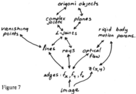
The advantages of using several hierarchical levels of abstraction in vision are: (l) the interaction between levels is simplified; (2) the same levels can be used by different feature spaces; and (3) more possibilities are allowed with the same number of units. Abstraction levels do not mean that high-level descriptions cannot influence low-level descriptions, or that the entire computations are not carried out in parallel. Rather, each descriptive level can only influence nearby levels. In Sabbah [1981], the limitation is to levels directly above and below. Other levels are influenced indirectly. The implication for the constraint transforms, which specify the constraints between levels, is that the constraint relationships between levels involve only a few parameters. This is an especially important feature, since the space required by the constraint transform is exponential in the number of parameters, as are the sets {BK}. Different levels of abstraction have been used by [Hanson and Riseman, 1978). Examples using the constraint transform may be found in [Sabbah, 1981; Kender, 1978]. Sabbah uses four levels to recognize origami world figures. Figure 7 shows some organizations.
To show an example in detail, Kender's technique for detecting vanishing points in an images from oriented line segments [Kender, 1978] is described. Such line segments which are part of a given vanishing point form a rad1al field which emanates from the point. Different vanishing points have different sets of associated radial line segments (1-'ig. 8). The same situation occurs with respect to optical flow due to pure translation. If the objects in the image are stationary with respect to a translating observer, then the flow vectors will be emanating radially from a "focus-of expansion" (I .. OE) in the direction of motion. Objects translating with respect to the observ~r·s frame will P:?duce their own flow emanating from a different FOE (F1g. 8).
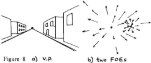
This example involves two levels of abstraction. The first transforms colinear edge segments into points (representing lines). Radial sets of edge elements correspond to circles through the origin in line-space. Thus the second transformation is between circles in line-space to points in radial -field space.
The first ievel is easy if a (r,O) line space is used where
Since an edge element has direction a (Fig. 9), each such element maps onto precisely one point in (r,IJ) space: (x cosa + y sina, a). Thus the constraint transform, in the notation of Section 3, is:
<(x,y,a{x,y)), {r,IJ), (0 = a; r = x cosa + y sina)>.
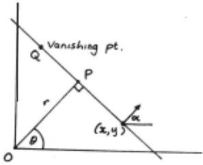
Now maxima in C{r,O) correspond to lines in the image. Also, radial lines will form a circle of local maxima in (r.tJ) space. To see this note that the triangle OPQ in Figure 9 is always a right triangle, and therefore OQ must be the diameter of a circle. Note that this circle is constrained to go through the origin so that its diameter must be on the line
r/2 = a coso + b sino
where (2a,2b) is the location of the focus of expansion (or vanishing point). Thus the second transform is
Implementation in Parameter Networks
The earlier definition of the constraint transform assumed that the measurements ak all had confidence equal to unity. With higher level of abstraction constraint transforms, this may no longer be the case. This is easily handled by keeping track of the confidences in the set Bk, i.e.,
Then H(b) is the sum of the confidences associated with the value b in UkBk.
6. Focus-of-Attention
The earlier examples of intrinsic image to feature space transforms used constraint transforms between just two spaces. Two main issues arise when multiple feature spaces are involved. First, when multiple constraint transforms are invoked in parallel to detect a segment with multiple features, some modalities may not have a high-confidence unit. This problem is solved via the mechanism of a context constraint transform which allows an ambiguity in one space to be resolved by another. Second, there is the problem that occurs in associating multi-modal features with a more abstract segment. How can one keep track of spatial registration and avoid exponential growth in the number of units? This problem is solved by a tuning mechanism, which assumes the high confidence units are sparsely distributed.
6.1 Spatial Context
If a unit has multiple spatially registered features, these can be detected by applying two different sets of constraint transforms. The constraint transform defined in Section 3 is bottom-up: points in the intrinsic image space determine plausible sets of points in feature space. The complementary transform is top-down: points in feature space determine plausible sets of points in intrinsic image space. Formally, given a set {bk} E B, compute
H(x) is the number of times the value a(x) occurs in UkAk. The mapping which defines H(a) is likely to be one to many and furthermore, for a given feature, different bks should give rise to disjoint subsets of A. Owing to this last point, it is intuitively appealing to deal with Ha(x) which is simply the sum of the confidences of different values of the parameters a1,a2···· which are at the same spatial location x,y, i.e.,
An Example
Consider an image of a red spot on a green background, where the spot takes up one-third of the image pixels. Then the transform C(b) where b = r,g,b has two peaks and is zero everywhere else, i.e., for four-bit color scale accuracy
Now consider b1 = {15,0,0) and compute C(a,x). This is given by
A point in A represents the single color red and so H(x) in this case is
The transform H(x) is called the spatial context transform for reasons that will become more apparent when we discuss focus of attention. The effect of this transform is to place an imaginary filter or mask in front of the sensors. In the above case, only sensors that are spatially registered with RED sensors would receive input.
6.2 Subspaces and Sequencing
A segment in an image is ideally represented as a conjunction of constraint transform maxima. Each set of maxima corresponds to an organization with respect to a given modality: color, velocity, etc. The previous section showed how the parallel generation of these maxima could be used to discover regions in the image corresponding to multi-modal units. Unfortunately, this technique will usually be inadequate because the unit is not manifested as a clear maxima in all the modalities. As an example, consider a light-blue, moving unit, against a background of other units, none of which are light-blue, but which are moving. In the color space, the unit is clearly revealed; light-blue units have high confidence values (Fig. 10). In velocity space, however, there may be no clear maximum owing to the presence of other moving units.
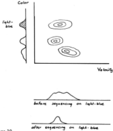
The fundamental problem is that each modality consists of a projection of multi-modal feature space. In the high dimensional space consisting of the concatenation of all the individual dimensions of each modality, each unit would appear as a distinct maximum. The visual system model is structured to examine only the subspaces of the individual modalities. The principal reason for this is economy; the space requirement increases exponentially with the number of modalities.
This problem can be surmounted if the different parameter spaces are examined sequentially. First the parameter spaces are examined for maxima. The most distinct maxima is picked and its inverse constraint transform, C(x), is generated. This transform can be usd to block input from sensors positioned at its low confidence values. To see how this might work, let us reconsider the previous example of the light-blue, moving unit. In color space there is a clear maximum corresponding to light·blue. ~!'his value is used to generate CJight-blue(x) and block mput from all sensors that are not spatially registered with hght-blue color input. The net effect is that in velocity space there is now a clear maxima as input from other units has been blocked. This technique is similar to that of Sec.;tion 4; the differences are: (1) feature spaces are multi· modal, and (2) the use of the masking effect of spatial context.
6.3 Multiple, Spatially·Uegistered Features
Sequencing solves the problem of building up coherent groups of features, but poses other problems. For example, if the "blue," "moving," "horizontal" object were a "frisbee," one would like this percept to be triggered via a constraint transform. However, in the sequencing example, there is initial evidence for all light-blue objects, and this is a very large set. Worse, the percept "frisbee" could be triggered by non-spatially registered groups of "blue" and "moving" inputs. There is a solution to these problems if one assumes that, in general, actual occurrences of features will be sparse. In other words, in a given image there should not be two very similar colors associated with different objects. If there are, our constraint transform model will only be able to concentrate on one of them at a time.
The solution is due to [Feldman and Ballard, 1981]. It is developed here, in terms of the constraint transform formalism, in three steps. First, we formally concatenate parameter spaces. Next, we describe /ow-resolution concatenated spaces. Finally, we show how low-resolution parameter spaces can be tuned to specific parameter values.
Ideally, one could resolve the spatial registration problem by concatenating feature spaces. For example, concatenating color space with motion space leads to
where elements in the expanded space (bc,bm) E BcxBm are only included if the input features are spatially registered. While this is simply described in symbolic form. it is also impractical since the parameter spaces for the combined-modality elements are impractically large. A partial solution to the size problem is to decrease the number of parameter nodes. Let be· bm · be values for color and motion parameters respectively in low-resolution spaces. Then the low resolution constraint transform is given by
where the bounds De and Dm are larger to account for the lower-resolution in parameter space. The grain of the low resolution space can always be chosen to make the transform practical in terms of space. However, now groups of parameters that are sufficiently similar may be transformed into the same parameter node via Eq. (5.1). To resolve this problem use a two-tiered transform, consisting of high-resolution single-modality transforms and low resolution multi-modality transforms. Using the single modality transforms, select maxima {be ·J and {bm ·J such that
and
These values are then used to tune the low-resolution constraint transform, i.e.,
Thus the low resolution transform can be tuned to count only a suQset of the high resolution parameter nodes. The drawback of this technique is that it can only respond to a single value of (bc,bm) in each range {be + .56c, bm + .56m}. Thus either the high confidence parameter nodes must be sufficiently sparse, or only one of the confusion classes can be examined at any one time. This disadvantage is outweighed by being able to detect spatially-registered features and thus circumvent the more severe problem discussed earlier.
7. Tight Coupling
Most of the previous examples imply that the various constraint transforms are relatively independent. That is, once the intrinsic images are computed, the transforms can be computed. The general case is that this is not true; the intrinsic image contains global parameters which must be computed using constraint transforms. Since the constraint tra.nsform required an intrinsic image it might seem that neither could be computed. In fact, both the constraint transform and the intrinsic images can be computed by incorporating the constraint transforms into the parallel· iterative scheme used to compute the intrinsic images. If the combined problem is well-conditioned: 1) the partial result for the intrinsic image will be sufficient to produce a partial result for the constraint transform, and vice versa; and 2) this process of using partial results in a parallel-iterative manner will converge. We term this interdependence tight coupling and illustrate it with an example.
The example shows how a surface orientation intrinsic image can be computed from intensity information. This example seems paradoxical at first since to compute surface orientation one must know the location of the source of illumination and vice versa. However, both these computations can be conducted simultaneously with the partial result for the surface orientation helping the illumination angle determination, and the partial result for the illumination angle helping the surface orientation determination. The illumination angle is determined by a constraint transform. Rather than being an isolated example, tight coupling is believed to be the general case. Extending the scope of the parallel-iterative computation is the general solution.
7.1 Shape from Shading by Uelaxation
Given the orientation of a surface with respect to a viewer, its reflectance properties and the location of a single light source, that the brightness at a point of the viewer's retina can be determined. That is, the reflectance function R(O,rp,Os·~~'s), where O,rp and Os·'l's are orientations of the surface and source respectively, allows us to determine l(x,y), the normalized intensity in terms <>f retinal coordinates [Horn and Sjoberg, 1978]. The form of R is assumed to be known. However, the perceptual problem is the reverse: given l(x,y) and R{.,.), determine o(x,y),rp{x,y) and Os·~~'s ·
In general, the problem of deriving O(x,y),<p(x,y) and Os·'l's is underdetermined. However, lkeuchi [1980] showed that the surface could be determined locally once Os'l's was specified. This method has been extended [Ballard, 1981 b] to the case where Os·'l's is initially unknown .
To calculate Us and 'l's· assume u and 'P are known and use a constraint transform technique. First form an array H[Us·'l''sl of possible values of Os and 'Ps initialized to zero. Now solve the reflectance equation for 'Ps. The constraint transform technique works as follows. For each surface element O,<p, and for each Us calculate 'Ps and increment H[Os·'Psl· i.e., H[Os·'l'sl : == H[Os,'Psl +I . After all surface elements have been processed, the maximum value of C corresponds to the location of the point source. In [Ballard, 198lb] it is shown that calculation of the source location can proceed in parallel with that of O(x,y) and <p(x,y) and that the two calculations will converge.
Results for the two ljimensional case are shown in Figure l 1 for the case of a small surface "bubble." Figure 1 l shows the surface convergence, as well as the convergence of the illumination angle.
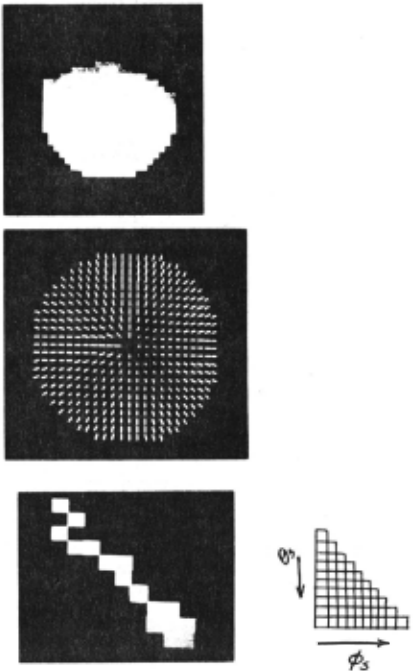
It is important to remember that the boundary conditions in this problem have been provided a priori; 111 this case they are the orientation of the surface at the boundary of the bubble. Generally, these will have to he Jetermined hy multiple intrinsic images relaxations, as mentioned in Section 2.
8. Discussion
This paper introduces a connectionist theory to show how parts of an image are seen as a segment. The focal point of the paper is the notion of constraint transform, which is a generalization of the Hough transform to non· analytical relations. A key contribution is the decomposition technique that allows high-dimensional constraint transforms to be partitioned into sequential groups of lower-dimensional constraint transforms.
The other important ideas in this paper are summarized in the introduction. Here we mention other ideas which do not fit easily under any one of the previous headings.
- The Intrinsic Image/Feature Space Decomposition. Distinguishing image fields and image features determines when relaxation is the more important tool and when the constraint transform is more important.
- Unit/value. Reducing the underlying primitives to units of extreme simplicity allows the algorithmic determination of the connection patterns to represent m-ary relations.
- Massive Parallelism. Massive parallel computation reduces the need for sequential processing to more essential cases. ror example, in Section 5, sequential processing resolved real ambiguities in the input.
- Extensibility. The representation is very general, being m-ary consistency relations, and can be extended to other domains besides vision, or to arbitrary levels of abstraction within vision.
@inproceedings{ijcai1981p215,
  title     = {Parameter Networks: Towards a Theory of Low-Level Vision},
  author    = {Ballard, Dana H.},
  booktitle = {Proceedings of the Seventh International Joint Conference on
               Artificial Intelligence, {IJCAI-81}},
  publisher = {International Joint Conferences on Artificial Intelligence},
  editor    = {Patrick J. Hayes},
  pages     = {1068--1077},
  year      = {1981},
  month     = {8},
  note      = {Invited Talk},
  url       = {https://ijcai.org/proceedings/1981/215},
}
TY - CPAPER TI - Parameter Networks: Towards a Theory of Low-Level Vision AU - Ballard, Dana H. T2 - Proceedings of the Seventh International Joint Conference on Artificial Intelligence, IJCAI-81 PB - International Joint Conferences on Artificial Intelligence PY - 1981 SP - 1068 EP - 1077 UR - https://ijcai.org/proceedings/1981/215 ER -Copied
Machine-readable versions of this paper, for tools and AI agents:





