Hierarchical Description of Textures

I Introduction

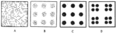
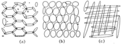
Texture carries useful information with which a vision system may discriminate objects and identify them. Thus it is necessary to describe textures compactly, for example, for scene analysis, analysis of aerial photographs, or diagnosis of medical images. Texture has been studied on at least two levels: statistical and structural [1]. On the statistical level, a texture is defined by a set of statistics extracted from a large ensemble of local picture properties. On the structural level, a texture is considered to be defined by elements which occur repeatedly according to placement rules. Roughly speaking, statistical methods are suitable for micro-textures and structural methods are suitable for macro-textures. There are at least four types of textures from the view of analysis. The model texture patterns are shown in Fig.l. Pattern A has many small texture elements in the image. So it can be described by global statistics without regard to the texture elements. Pattern B also has many small texture elements but they form local clusters. It is reasonable to regard clustered texture elements as regions and to describe the structure of those regions. Pattern C has comparatively large texture elements; it is reasonable to describe the structure of the texture

HIERARCHICAL DESCRIPTION OF TEXTURES

Fumiaki Tomita

Information Sciences Division Electrotechnical Laboratory 1-1-4 Umezono, Sakura-mura, Niihari-gun Ibaraki, 305 Japan

elements. Pattern D also has large texture elements but they constitute subpatterns. It is reasonable to . group such locally ordered texture elements and describe the structure of the subpatterns. In this paper, a system is proposed which analyzes textures statistically or structurally depending on their natures. Hierarchical descriptions of textures can be produced by the system.

II Overview ~ Analysis

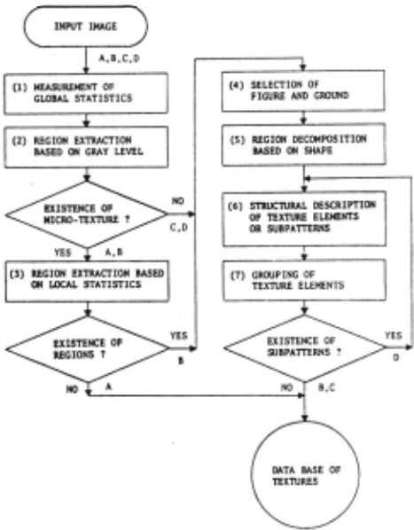
An overview of the flow of processing is shown in Fig.2.

(1) Measurement of Global Statistics

The system first describes every input texture globally to roughly classify it. It measures global gray level first order statistics and global edge statistics. They are adequate to describe textures like pattern A in Fig.l.

(2) Region Extraction Baaed on Gray Levels

The system extracts homogeneous gray level regions to try to describe a texture structurally. However, if too many regions are extracted or if regions cannot be easily extracted, this indicates the existence of micro-textures like patterns A and R in Fig.l.

(3) Region Extraction Based on Local Statistics

If the system recognizes the existence of micro-textures, it examines if the micro-textures constitute regions like pattern B in Fig.l. The system extracts such regions based on local gray level first ~rder statistics and local edge statistics. If there is no different region like pattern A in Fig.l, it stops analyzing a texture structurally.

(4) Selection of Figure and Ground

If there is more than one class of regions (which have been classified based on gray levels or local statistics), the system distinguishes ground regions from figure regions to examine only the structure of figure regions.

(5) Region Decomposition Based on Shape If the shapes of the figure regions are complex, the system decomposes them into regions of simpler shapes. The decomposed regions are atomic texture elements.

(6) Structural Description of Texture Elements

The system first classifies the atomic texture elements based on the shape, and next based on .the placement, and lastly computes the distributions of shape and placement of each class of texture elements.

(7) Grouping of Texture Elements

If there are locally ordered texture elements like pattern D in Fig.l, they are grouped into subpatterns. The system produces a structural description of the aubpatterns in the same way as it did for the atomic texture elements.

III Measurement !?.[ ~ Statistics

A number of statistical methods have been suggested for texture description [2]. Gray level first order statistics and edge statistics are used in this research. Edge statistics produce not only the same kinds of features as gray level co-occurrence matrices [3), which are moat popularly used second order statistics and evaluated better than some other statistics [4,5], but ala_o produce more structural features.

A. Gray Level !!!.!!.!. ~ Statistics

The system normalizes an input image with respect to gray scale changes so that the mean is 32 and the standard deviation is 8 anrl then COMputes skewness (the third order moMent) and entropy for a gray level histogram. Skewness is a measure of the symmetry of a histogram and entropy becoMes low when dense clusters appear in a histogram.

B. F.dge fLtatistics

An edge element has the descriptors of the edge value and the edge direction. The system uses edge elements whose edge values are locally maxiMal and greater than a threshold. It first classifies edge elements by recursively thresholding the descriptor histograms (6] and computes the next statistics for each class of edge elements.

(1) Density of Edge Elements

The density of edge elements is the number of edge elements per unit area and is a measure of texture coarseness [7]. The higher the edge density, the finer the texture. If the edge density is very high, the systeM can estimate the existence of Micro-textures in an image without directly counting the nuMber of texture eleMents in step 2 in Fig.2.

(2) First Order Statistics of Edge Values

The mean of edge values is a measure of contrast and the entropy of edge values is a measure of gray level randomness.

(3) First Order Statistics of Edge Direction

The directionality of a texture can be detected from an edge direction histogram (8]. The system computes a histogram of edge direction measured modulo n so that the distributions between n and 2n are the same as those between 0 and n. It first computes the entropy of the histograM to measure the edge direction randomness. Next, if there are 2N (N~l) clusters in the histogram, the system recognizes the existence of N directions and computes the mean and the standard deviation of each cluster between 0 and n. If there is only one cluster in the histogram, however, it represents no directionality in the texture.

(4) Second Order Statistics of Edge Direction

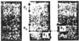
More structural features can be extracted from the second order statistics of edge directions [8,9). The co-occurrence probability of two edge elements with the same edge direction separated by a distance k along the edge direction (edge elements e 0 and e 1 in Fig.J) represents a linearity (k-linearity) of a texture. The co-occurrence probability of two edge elements with the same edge direction separated by a distance k along the direction perpendicular to the edge direction (edge elements e 0 and e 2 in Fig.J) represents the periodicity of a texture. The co-occurrence probability of two edge elements with the opposite edge direction separated by a distance k along the direction perpendicular to the edge direction (edge elements e 0 and e 3 in Fig.J) represents the size of texture elements. The system, however, measures only the k-linearity (k·S) since it measures periodicity and the size of texture elements more precisely in the later structural analysis of step

IV Region Extraction !!!!..!!!. .2!1 Gray Level

The system extracts homogeneous gray level regions to try to describe a texture structurally. There are two basic methods for region extraction: the thresholding method and the merging method. In the thresholding ~ethod, the gray level histogram of an image is computed. If there are some clusters in the hiatogr~, the image is segmented into regions so that the gray levels in a region belong to one of the clusters. The thresholding method, however, is too global; even though there are visually distinctive regions in an image, it is usual that no diatinctive:cluster appears in the gray level histogr~ because of the blurry effects. In the merging method, on the other hand, adjacent points in an image are merged into regions baaed on the gray level similarity. The merging method, however, is too local to evaluate the limit of the gray level similarity.

This paper proposes a merging-andthresholding method which combines the two methods to offsets the defects of each; the merging method is repeated until distinctive clusters appear in the gray level histogram and then the thresholding method is applied. The procedure of extracting regions from an input image 1(0) is as follows.

1. Set k·l.
2. Generate an image I(k) by merging adjacent points whose gray level differences are leas than k into regions and averaging the gray levels in the regions.
3. Compute the gray level histogram H(k) of the image I(k).
4. Teat whether distinctive clusters exist in the histogram H(k). If so, go to step 5), or else set k·k+l and go to step 2).
5. Threshold I(O) by the gray levels between the clusters in the histogram H(k) in order to extract regions.

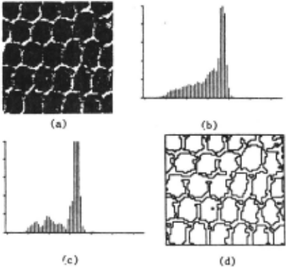
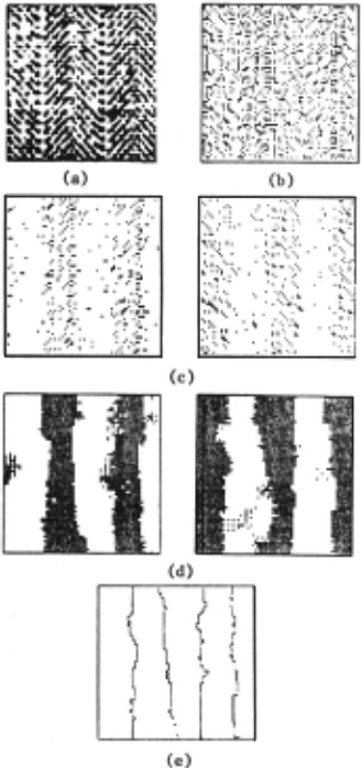
For example, the gray level histogram H(l) of an image in Fig.4(a) is shown in Fig.4(b). No separable cluster exists in it. Merging by k·5 makes two separable clusters appear in the hiatogr~ H(5) as shown in Fig.4(c). As a result, the image are segmented into regions by threeholding aa shown in Fig.4(d).

V Reaion Extraction !!.!!!!. .2!1 Local Statistics

If too NAny region· are extracted or regions are extracted by too large a k value, the system recognizes the existence of micro-textures in an image. In such a case, it extracts regions baaed on the local gray level first order statistics and the local edge statistics. First, it computes the mean gray level and the density of each class of edge elements (which have been classified in section III.B) in the neighborhood of every point. Next, it extract regions baaed on the local statistics computed [10]. For example, edge elements of an i~age in Fig.5(a) are shown in Fig.5(b). In this case, the edge elements are classified into two classes by thresholding the edge direction hiatogra~ as shown in Fig.5(c). Then the system computes the local density at every point for each class of edge ele~ents and it extracts regions of high edge density as shown in Fig.5(d). J~stly, it extarcta regions in Fig.S(e) by superimposing regions extracted separately in Fig.S(d) and by merging small overlapping regions to neighboring large regions. If the system cannot extract such different regions, however, it stops analyzing a texture structurally.

VI Selection !!! Figure .!.!!!!. ~

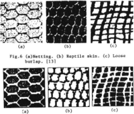
If there is more than one class of regions (which have been classified baaed on gray levels or local statistics), one of them can be regarded as the ground of an image. If an observer has knowledge about the objects in the image, he can recognize the regions corresponding to the objects as a figure. On the other hand, if he knows nothing about the objects, he cannot determine which regions correspond to the figure of the image. Psychologically, however, regular regions are apt to be the figure of the image. In the learning phase of our system, a user can arbitrarily select a ground region class. Otherwise, the system ranks region classes according to the regularities of the shape and the placement Which can be measured in step 6 in Fig.2. For example, selected figure regions of the images in Fig.6 are shown in Fig.7.

VII Region Decomposition ~ ~ Shape

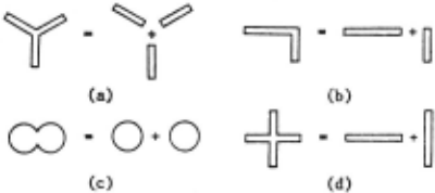
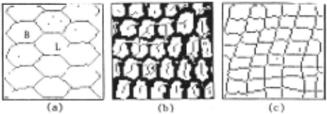
If the shape of a figure region is complex, the region is decomposed into regions of simpler shapes according to Gestalt psychology. For example, the region in Fig.S(a) is decomposed into three branching regions, the region in Fig.S(b) is decomposed into two linking regions, the region in Fig.S(c) is decomposed into two overlapping regions, and the region in Fig.S(d) is decomposed into two crossing regions. In our system, the shape complexity of a region is evaluated by the connectivity-preserving skeleton [11]. For example, the skeletons of the figure regions in Fig.7 are shown in fig.9. Each point on ths skeleton has the distance value from the boundary of the region. Since the connectivity of a region is preserved in the skeleton, the segmentation of the skeleton corresponds to the segmentation of the region and the merging of the skeleton corresponds to the merging of the region.

(1) Branch

If the skeleton branches as shown in Fig.S(a), the skeleton is segmented at the junction. However, there is a problem of spurs appearing in a skeleton. Spurs occur through the effects of small fluctuations of the boundary of a region. They make unnecessary branches. Since the distance values along a spur monotonically decrease from the junction, the branches whose distance values monotonically decrease are deleted. Let W(O), ··· ,W(N) denote the distance values of the skeleton S·P(O), ··· ,P(N). If the skeleton satisfies the following conditions, the points except P(O) are deleted.

(2) Link

If the skeleton bends sharply as shown in Fig.9(a), the curvature at a bending point is locally maximal; the skeleton is segmented at a point of a locally maximal curvature. Let C(O) ····· c(N) denote the absolute values of k-curvaturea of the skeleton S·P(O) ····· P(N). The skeleton is segmented at a point which satisfies the following conditions,

(3) Overlap

If objects overlap. a locally minimal distance value appears around the overlapping portion of the corresponding skeleton as shown in Fig,9(b); the skeleton is segmented at the point of a locally minil'l&l distance, Let 1~(0) · ··· 0W(N) denote the distance values of the akeleton S·P(O) ····· P(N). The skeleton is segmented at a point which satisfies the following conditions.

(4) Intersection

A cross-shaped skeleton is first decomposed into branching skeletons at the junctions. However. if the branching skeletons are linearly connecting as shown in Fig,9(c) 0 they are merged into one skeleton. Let SJ·PJ(l) 0PJ(2),,.. and s7·P ;· (1) 0 P2 (2) ·... denote a pair of branching skeletons. where the distance between P1(l) and Pz(l) is within a threapold. If the angle between P1(k)P1(1) and Pz(l)Pz(k) is leas than a threahold 0 the two skeletons are merged into one skeleton.

The system labels decomposed skeletons differently and expands t·hem to regions. As a result. decomposed regions are extracted, The decomposition makes description of textures more powerful than before in [12].

For example, the decomposition of Fig,7 are shown in Fig,lO. Those regions are atomic texture elements, regions in decomposed

VIII Structural Description £[ Texture Elements

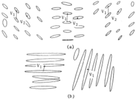
The system produces a structural description of atomic texture elements, Firat, it further classifies texture elements baaed on shape. (They were already classified baaed on gray level or local statistics.) It measures such shape descriptors of a texture element as the size. the area, the direction of the major axis. and the ratio of the minor axis to the major axis [12]. (The last three descriptors can be used to approximate the shape of a region by an ellipse as shown in Fig,lO,) The system classifies texture elements by recursively thresholding the shape descriptor histograms and it computes the mean and the standard deviation of the shape descriptors for each class of texture elements. Fig,ll illustrates the result of classification of texture elements in Fig.lO.

Next. the system classifies texture elements baaed on placement, For each texture element in a class i, it computes the relative position vectors V 1 (i)· {q (i) .91 (i) } and V z(i)· {r z(i) ,9 z(i) } to the nearest and the second nearest texture elements in the same class i and the relative position vector V(i,j)·{r(i,j),9(i,j)} to the nearest texture element in other class polar coordinate and ~ However. there are some them. j 0 where (r,8) denotes a is measured modulo n, conditions in computing

(1) If r1(i)·r2(i), the vector whose 9 is the nearer to 0 is set to V1(i) and the other is set to V2(i),

(2) If rz(i)>2r1(i) or 91(i)·92(i) 0 the second vector V2(i) of the texture element is ignored,

For example, relative position vectors of texture elements are shown in Fig,ll. The texture elements in Fig,ll(b) satisfy the condition (2) and have only one relative position vector, respectively,

Then the system classifies texture elements by recursively thresholding the histograms of rJ(i), 91(i), r 2(i), and 92(i), Lastly, it computes the means and the standard deviations of the relative position vectors for each class of texture elements as the placement rules {RJ(i),R2(i)l and {R(i,j)l (i~j).

IX Grouping of Texture Elements

If there are locally ordered texture elements, they are grouped into subpatterns. The system groups texture elements using the placement rules {RJ{i) 1 R2{i)} or {R(i,j)} as follows.

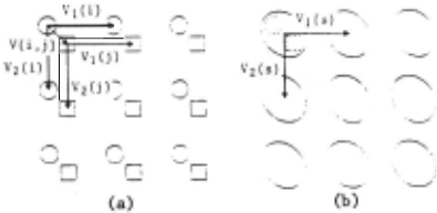
(1) If R!(i)·Rl(j), R2(i)·R2(j), and 2r(i,j) <r 1 {i) {r denotes the mean of r), the placement rule R{i,j) is used to group a pair of texture elements, one in class i and the other in class j. For example, let texture elements in class i (0) and class j (D) have a relative position vector V(i,j) which belongs to R(i,j) as shown in Fig.l2(a). Every pair of texture elements whose spatial relation belongs to R{i,j) is grouped into a aubpattern as shown in Fig.l2{b).

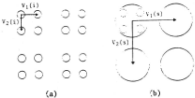
{2) Otherwise, the placement rules RJ(i) and Rz{i) are used to group texture elements in class i. For example, let every texture element have relative position vector V1(i) and Vz{i) which belong to RJ(i) or R 2 (i) as shown in Fig .· 13(a). The texture elements whose spatial relations belong to RJ(i) or Rz(i) are grouped into subpatterns as shown in Fig.l3(b).

The system produces the structural description of subpatterns in the same way as it did for atomic texture elements. If all the texture elements in one class are grouped into one group, however, it represents that no subpattern exists. texture elements i n Fig.lO(b) and grouped into one group respectively. For example, Fig.ll are

X Conclusion

A system is proposed here which analyzes texture statistically or structurally depending on the nature of textures. The system first describes a texture globally by gray level first order statistics and edge statistics to roughly classify it. Next, it produces a hierarchical structural description if pos~ible. The texture is described at the top level by subpatterns arranged according to placement rules. Each subpattern is also described by subpatterns at a lower level in the same way, and so on. At the bottom level, each subpattern is described by atomic texture elements. Atomic texture elements are locally homogeneous regions of simple shape. The shape descriptors of an atomic texture element or a subpattern are the size, the area, the direction of the major axis and the ratio of the minor axis to the major axis. The placement rules measured are relative position vectors between texture elements or subpatterns.