Determining Velocity Map By 3-D Iterative Estimation

DETERMINING VELOCITY MAP BY 3-D ITERATIVE EST1MA1'ION

Masahiko Yachida

Fachbereich Informatik, Universitaet Hamburg (on leave of absence from Dept. of Control Engi, Osaka University)

I INTRODUCTION

Velocity information is not only important for determining velocities and trajectories of objects but also important as a cue for image segmentation. It may be used to link adjacent but visually dissimilar surfaces or to divide surfaces not easily separable by static criteria alone[l].

A straightforward approach to obtaining velocity information is to find and track prominent features by a matching method from frame to frame[2,3]. These methods can estimate velocities of prominent points accurately; however, a problem of these methods is that velocities of only a sparsely sampled set of points can be obtained, which are not dense enough to be useful for tasks such as image segmentation.

Another approach uses the fact that for images of moving objects the spatial and temporal intensity changes are not independent of each other and satisfy a

relation

Vx*Gx+Vy*Gy=-Dt (l)

Here, (Vx,Vy) are the two components of the velocity vector, (Gx,Gy) represent the two components of the spatial intensity gradient, and Dt represents the gray value difference between consecutive frames, at a point (x,y).

Since the single constraint of Eq. (1) does not allow one to determine both components (Vx,Vy) of the velocity, additional assumptions are necessary. Cafforio and Rocca[4] and Fennema and Thompson[S] assumed that the velocity is constant within a region corresponding to the image o f a moving object, and applied a clustering approach to determine the dominant velocities in the scene. By this global method, they obtained accurate velocities of objects; however, with that assumption, the method is applicable only to objects which translate parallel to the image plane. Horn and Schunck[6] studied a more general assumption; namely that the velocity varies smoothly. This assumption is interesting because it constrains the

variability of velocities between neighboring points estimate the velocity local computation. seems to become more if we have some velocities. and allows one to of each point from However, the method efficient and reliable initial estimates of There has been no attempt to try to combine or relate the matching method by which accurate estimation of velocities (although of only a sparsely sampled set of points) are obtained and the nonmatching method by which velocities of a dense set of points can be estimated, but additional constraints are required. In this communication, we propose an approach which uses the velocity estimates of the prominent feature points as reliable initial estimates of velocities and propagates them to other points using the constraint relation between the neighboring points. The veloc ities estimated by the above method based on the local data may have errors caused by noise. To reduce or eliminate these estimation errors, we propose an iterative scheme which corrects and modifies the estimation from the velocity values of the spatial and temporal neiborhood of a point.

II VELOCITY ESTIMATION FROM PROMINENT POINTS BY PROPAGATION

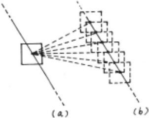
Local computation of the velocity is, in general, not possible since Eq. (1) does not a llow one to determine both components of the velocity. This will be clear from Fig.l where (a) shows a part of an object in the previous frame and (b) shows the same part in the next frame. It is not possible to determine the velocity of the local area enclosed by the rectangle since it can correspond to many areas in the next frame. However, as shown in Fig.2, it is not difficult to establish correspondences between the prominent feature points. Once these have been established, it is not difficult to establish correspondences o f other points because the correspondenc es of the feature points constrain possible correspondences of other points, provided we can assume that the object is rigid and

thus velocities vary smoothly.

Based on the above idea, we study, in this correspondence, the propagation of the velocity estimates from the prominent feature points using the constraint relation between the neighboring points. As we also assume that the velocities vary smoothly, we follow Horn and Schunck[6] and the constraint relation can be written as E2=SQR'l'[ (Vx-Vx t + (Vy-Vy f ]===> Minimum (2) where (Vx,Vy) represents the velocity of a point (x,y) and (Vx,Vy) represents the average velocity of its neighboring points. For each point (x,y), we have the relation {1). Because there are estimation errors caused by noise, we rewrite it as

El=Vx*Gx+Vy*Gy+Dt ===> Minimum (3) 2 By minimizing the total error E.2=a.2 *El.t +E2 (a: constant), we can derive the following two equations[6]: 2 2 Vx=Vx-Gx*(Gx*Vx+Gy*Vy+Dt)/(a +Gx +�~) Vy=Vy-Gy*(Gx*Vx+Gy*Vy+Dt)/(a 2 +Gx2 +Gy 2 ) (4) Velocity estimation are propagated from the prominent points in the image using Eq. (4) as follows.

1. Estimate the neighboring points in the image by Eq. (VX,vy) use (Vx,Vy) velocities of the ot each prominent point 4, in this case, for of the prominent point.

2. Estimate the velocities of neighboring points of those velocities have been estimated at previous propagation. In this (VX, Vy) is calcurated from a neighborhood of those points velocities have been estimated in previous estimation. the whose the case, 5*5 whose the

3. Iterate the propagation until velocities of all the points in the image have been estimated.

Ill ESTIMATING THE SWDENC"EsVELOCI'l'Y IN

Let us define the I(x,y,t),t=l, ... ,N. sequence of image sequence as Then we can obtqin a velocity maps V(x,y,t),t=2, ... ,N by the method described in the previous section, such as V(x,y,t) from the two images I(x,y,t-1) and I(x,y,t). However, when we have estimated the velocity V(x,y,2) from the first two frames I(x,y,l) and I(x,y,2), it is more efficient to predict velocity distribution in the next frame, V (x,y,3), from the velocity map V(x,y,2), and use the prediction map V (x,y,3) in order to estimate the velocity of the next frame[7], , if we can assume that velocities vary smoothly between consecutive frames[6]. This constraint between neighboring points in consecutive frames can be represented by EQ. (2) where, in this case (VX,Vy) is the average of velocities of neighboring points in the prediction map and {Vx,Vy) is the velocity of the current frame to be estimated at the point (x,y). Therefore we can estimate the velocity V(x,y,t) of the t-th frame from the velocity V(x,y,t-1) of the (t-1)-th frame using Eq. (4). This is iterated until the N-th frame has been estimated.

IV ITERATIVE CORRECTION OF VELOCITY ESTIMATION BY 3-D NEIGHBORs-

We have estimated velocities V(x,y,t),t=2, ... ,N, of each point for the sequence of images. These velocities, however, have been estimated by local computation, and therefore may have estimation errors caused by noise. To eliminate or reduce these estimation errors, we propose an iterative method which corrects and modifies the estimation from the velocity values of spatial and temporal neighborhood of a point. We assume here that velocities vary smoothly between neighboring points and between consecutive frames. Then, Eq. (2) holds for the spatial and temporal neighbors. Then, we correct the estimation of a point (x,y) in the t-th frame by the average velocity {Vi,Vy) of neighboring points (5*5 points) in the (t-l)th , t-th and (t+l)th frames (in total 5*5*3 points), using Eq. (4). We obtain the newly estimated velocities at every point for every frame,t=2, ... ,N. This newly estimated sequence of velocity maps, V(x,y,t),t=2, ... ,N), is again used as input for the next iteration. This process is iterated until major changes do not occur in the sequence of velocity maps.

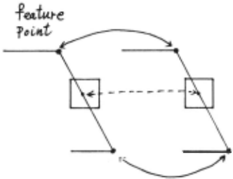
Fig.3 shows some examples of the results.

ACKNOWLEDGEMENT

The author thanks H.-H. Nagel for his support, encouragement and discussions for this work, B. Neumann for very nice introduction to the laboratory facilities and software and members of Kognition Group of Universitaet Hamburg for their friendly and timely suggestions to the laboratory facilities a ~d software. He also thanks to Humboldt Fou Jdation for their hospitability ,under whose support this work was performed.