
Shape from Shading for Surfaces with Texture and Specularity
Proceedings of the Seventh International Joint Conference on Artificial Intelligence. Vision: 3-d. Pages 652-656.
© 1981 International Joint Conferences on Artificial Intelligence
Abstract
The primary focus of this work is to experimentally explore a method for determining three dimensional surface shape from intensity information. A method is developed, using existent theory, for determining the shape of visually textured surfaces exhibiting varying degrees of specularity. The photometric~ is extended to four source photometry as the basis for this work. The reflectance map approach for determining surface normals is shown to be of 1 ittle value in this context and a more direct method of computing these normals is used.
- Horn, Shading Computer 1975.
- B. K. P., "Obtaining Shape from Information", in The Pyschology of Vision, P.H. Winston (ed.), McGraw-Hi 1~ 2. Horn, B. K. P., Understanding", AI Memo Laboratory, August 1975. "Image Intensity 335, M.I.T. AI 3. Horn, B. K. P., "Sequins and Quills Representations for Surface Topography", AI Memo 536, M. I .T. AI Laboratory, May 1979. •
- Horn, B. K. P. And Sjoberg, R. W., "Calculating the Reflectance Map", AI Memo 498.
- M. I .T. AI Laboratory, October 1978.
- lkeuchi, K. And Horn, B. K. P., "An Application of the Photometric Stereo Method", AI Memo 539. IJCAI
- M. I .T. AI Laboratory, August 1979.
- Newman W. M. And Sproul I R. F., Principles of Interactive Computer Graphics, McGraw-Hi I 1, New York, 1979. 6 57
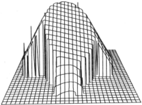
- Figure 7. Square pyramid plotted results. Surface generated from measured intcnsltv values. Viewpoint conrdinatcs: (-15,-15,15).
- Silver, W. M., "Determining Shape and Reflectance Using Mutiple Images", M.S. Thesis, M.l .T. AI Laboratory, May 1980.
- Woodham, R. J., "Reflectance Map Techniques for Analyzing Surface Defects in Metal Castings", AI-TR-457.
- M.l .T. AI Laboratory, June 1978.
- Woodham, R. J., "Photometric Method for Determining Surface Orientation from Multiple Images", in Optical Engineering, Vol 19, No.I, pp. 139-144, Jan/Feb 1980.
- Coleman, E. N. And Jain, r., "Obtaining 3- Dimensional shape of textured and specular surfaces using four source photometry TR No. CSC-81-020, Dept.
References were extracted automatically from the PDF and may contain errors.
Full text extracted automatically from the PDF; figures, tables and equations may differ. The PDF is the version of record.
SHAPE FROM SHADING FOR SURFACES WITH TEXTURE AND SPECULARITY
by
E. North Coleman Jr. and Ramesh Jain
Department of Computer Science Wayne State University Detroit MI 48202
Specular reflection, or high! ights, appear on a surface when the angle between the viewer and source of i 1 lumination is bisected by the surface normal. By producing a mirror-! ike reflectance off an object's surface, specularity causes measured intensity values to be higher by the magnitude of the specular component . Although attempts have been made to account for specularity in reflectance functions and reflectance maps, these functions are contrived for certain cases and fai 1 to solve the general problem. In this paper, visual texture 'is considered as a pattern or variance of intensity appearing on an object surface.
The motivation behind this paper is to adapt multiple source photometry to surfaces vary i ng i n both specularity and visual texture. Toward this end it wi I I be shown how surface normals can be computed by solving sets of simultaneous 1 inear equations. Detailed by Woodham [9] this method can be used on textured surfaces . Furthermore , it wi II be shown how a fourth source of i I lum i nation can be used to detect specular reflection . Once discovered, the specular component can be removed from the computation of a local normal vector.
l.!. SURFACE SHAPE FROM INTENSITY
U Definitions
ABSTRACT
The primary focus of this work is to experimentally explore a method for determining three dimensional surface shape from intensity information. A method is developed, using existent theory, for determining the shape of visually textured surfaces exhibiting varying degrees of specularity. The photometric~ is extended to four source photometry as the basis for this work. The reflectance map approach for determining surface normals is shown to be of 1 ittle value in this context and a more direct method of computing these normals is used.
.!. INTRODUCTION
Several methods are avai !able for obtaining depth information for surfaces. These methods are divided into what Woodham [8] refers to as direct methods and indirect methods. Direct methods try to measure range (distance) directly. Indirect methods attempt to determine distance by measuring parameters calculated from images of the i I luminated object.
One indirect method for obtaining surface shape is by analysis of the radiometry of image formation[l-5,7-9]. Commonly known as shape from shading, this method can be applied wherever the direction of incident i I lumination is known and/or can be controlled. It is this technique which is the subject matter of this paper.
Horn [1] showed how shape could be determined by solving non- I inear, first order partial differential equations to find components of the surface gradient. While the gradient could not be determined locally, numerical integration of the equations permitted characteristic curves to be traced out on the object surface. Woodham [8,9] suggested photometric ~ for locally determining surface gradients using multiple sources of illumination.
Multiple source photometry is usually implemented using one reflectance map for each image. To initialize such a reflectance map, the system is calibrated using a sphere having a constant surface reflectance factor. Silver [7] has shown this method to be very effective in solving for shape with uniform matte surfaces.
' Ill-i-s-work~-~- p.~rt·f;;·(fy supported hy Nat ion a 1 Sc i ence Foundation under the Grant No. MCS-8100148.
A surface photometric function Q(i ,e,g) for a single source can be defined in terms of the incident angle (i), emittance angle (e) and phase angle (g). As such, the angles quantify the relationship between the source vector, view vector and surface normal vector . Each of these vectors can be written in gradient space
coordinates as
V K (0,0,-1)
(view vector) 2.3
S K (ps,qs,-1) (source vector) 2.4
From the reflectance map, Woodham [8] i I lustrates how a single intensity value restricts the p and q values of the surface normal to a part i cuI ar i so-br i gh tnes s contour. The goa 1 ·of shape from shading is to isolate which (p,q) value on the contour is the correct surface gradient . l...,l ~ Source Photometry
Once a reflectance map is established, the process of determining the shape of sample objects can begin . When a single source of illumination is used, a single image intensity value maps into many poss ible surface orientations. To resolve these ambiguities, algorithms developed to solve for surface shape, using a single source, assume certa i n surface constraints. Woodham [8] assumes surfaces to be uniform, matte, convex and smooth with cont i nous first and second partial derivatives. From this assumption, his iterative algorithm propagates these constraints back and forth unti I converg i ng on a solution for the entire surface.
~Multiple Source Photometry
Photometric stereo, in essence, is multiple source photometry where two or more images of an object are obtained from the same viewpoint . In each image the object is i I luminated from a d i fferent direction by a single source. This gives rise to an-tuple of intensity values for each (x, y) point on the surface .
The first step in multiple source photometry is to establish a reflectance map for each source of i I lumination . Then by tracing iso-br ightness contours for each source/intensity the intersec t ion point for alI contours can be found . This intersection . po int satisfies the intensity value requirements for each source and is thus the surface gradient at the corresponding image point (x' y) .
It has been shown [9] that a minimum of three distinct iso-br ightness contours is needed to find the surface gradient for a lambertian surface . This implies a minimum of three sources is needed . For the contours to intersect at single po int the source vectors cannot be colinear .
~Limitations of the Reflectance~
Given any reflectance map, shape can be determined for surfaces having photometric pr.operties identical to the surface used for reflectance map calibration. This impl i es that the specular component of all sample surfaces must be identical to that cast in the reflectance map. Add i tionally, specularity cannot be detected, as there is no indicator to show if an intensity value i s elevated due to specular reflection. Finally , when establ i shing a reflectance map the surface reflectance factor R i s made constant for all po ints on the surface . This forces a un i formity of i ntensity on the surface and prevents the application of reflectance map techniques to visually textured surfaces.
~A Direct Solution for the Lambertian Surface
To overcome the I imitations of reflectance map techniques, a solution for surface shape must provide both the surface normal and surface reflectance factor R at each point. For Lambertian surfaces this is
I (x,y) · R*cos( i ) · R*(S.N)/ISI\NI 2.6 If it is assumed the source and norma vectors, s and N, are unit vectors, the denominator for equation 2.6 becomes I. Equation 2.6 can now be written:
where (Sx,Sy,Sz) are the known components of the source vector and (Nx,Ny,Nz) are the unknown components of the surface normal.
Since 2.7 is an equation with three unknowns, a minimum of three sources and associated intensity values is needed to compute the surface normal at each point. Given the sources Sl, S2 and S3 along with intensity values 11, 12 and 13 at (x,y) a set of simultaneous equations can be

If we use Ms to symbo I i ze the source matrix, 1 the intensity feature vector at (x,y) and N the normal vector, equation 2.8 becomes :
To solve for the reflectance factor, R, and unit normal, N, e~ation_~.9 can be written as: R * N · tMs] T 2 . 10
Using equation 2.10 the surface normal can be computed directly from a triplet of intens i ty values I and the inverse of the source matrix Ms. For Ms to have an inverse the source vectors Sl, S2 and S3 must not be colinear.
The reflectance factor, R, can be found simply by taking the magnitude of the right side of equation 2. 13. This is because the surface normal, N, is of Ur) i t length.
Once the reflectance factor is found the unit normal can be computed ~:
Using 2. 12 a 11 three components of the unit surface norma l can be found. It is necessary to compute all three components as the unit surface normal wi 11 not necessarily have Nz · -1. £..:2 Hand I ina Vi sual Texture
By solving for the unit normal vector in the previous section, it has also bee!) shown that the surface reflectance factor R can be determined locally at each (x,y) point on a surface. This implies that R need not be constant over the surface. Regardless of how R var .. ies, it can sti II be computed at each point using equation 2. 11.
Visual texture can be thought of as a pattern caused by variance in the surface reflectance factor from po i nt to point on a given surface. Indeed, shading models have been developed in computer graph ics uti 1 izing a variable reflectance factor to effect surface in tens i ty[6] . Thus, it can readily be seen that apply i ng equation 2.10 allows surface normals to be computed when the object is visually textured, as R i s computed locally at each point.
~Overcoming Specular Distortion
One method of overcoming specularity problems in a shading model is by incorporating terms into the reflectance function to account for the specu 1 ar component. Bu i ·I ding such terms into the reflectance function, however, ties the model to a single expression of specularity. A more flexible method is needed which enables the specular component to vary from one surface to another or even across the same surface.
As was shown in section 2.5, three sources are a II that are needed to unique 1 y determine surface normals for a Lambertian surface. If, however, a point on the surface is subject to specular reflection from one of the three sources, the computed normal vector wi 11 be incorrect due to an elevated intensity value. By adding a fourth source, it becomes poss i b 1 e to compute a set of four surface normal vectors for each point; i.e. one normal for .each permutation of three intensity values. It is this redundancy which allows tagging and removal of the specular source.
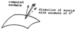
To see how this is accomplished first assume we are given four measured intensity values nt a point (x,y) on a surface; one intensity from each source/image. If none of the intensities has a specular component, the resulting four surface normals wi II appear as in Figure la. On the other hand, suppose the intensity value from an arbitrary source/image (source four in this case) contains a specular component elevating its value. The resulting four normals computed will be similar to the case illustrated in Figure lb.
It can readily be seen that there is a greater deviation in both direction and magnitude of the vectors in Fig. lb than those in Fig. Ia. Three of the norma l vectors in Fig. lb (the three computed using source four) are affected by a specular component. Because of this reason, their magnitudes, R, are greater and they are skewed more in the direction of the specular source.
A method can now be developed to eliminate specular effects using a thresholding procedure. The first step is to compute a relative deviation in the surface reflectance factor R at each point on the surface . This can be done using the ~
formula: ) Rdev · l ~(R i -Rmean) I (4*Rm in) 2. 14 where Ri is each re~ fectance factor computed at (x,y) and Rmin is the smallest of these. A reflectivity deviation map can be displayed for the entire surface showing the reflectance deviation Rdev at each point. On a reflectivity deviation map, specular regions wi II be characterized by high reflectance deviation.
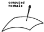
Fi~ur<· Ia. C:ompult·d normals at a single point on tilt· surfacP wh en no specular com pon<·nt Is pn·st·nt. Mt·an deviation among nornmls is snml I.
When computing surface normals, Rdev at each po i nt is checked against the threshold value Rt. If Rdev at a point is tess than or equal toRt, a specular component i s not considered pres·ent. The surface norma I is computed as the average of a II four normals calculated at this point. Rdev greater than Rt indicates a specular contribution at this point from one of the sources. To eliminate this specular component, the surface norma 1 is chosen as the computed norma 1 vee tor having the smallest reflectance factor .
In practice, the use of a threshold value wi 11 allow many surfaces to be analyzed successfully. A limiting factor is thai the specular component cannot be so great as to cause specular regions from two or more sources to overlap. This can be overcome to some degree by adjusting the angle of incidence for each source to prevent overlap.
Finally, the phase angles between all source vectors and the view vector must not be so large as to prevent al 1 four sources from contributing measurable intensity values throughout the arc of specular reflection. For most cases a phase angle of up to 60 degrees can be used (30 degrees above the image plane) but unde~ special circumstances the optimum source angles may have to be determined experimentally.
_1 _II_ ~ WORKING SYSTEM
A system consisting of specialized imaging hardware and a series of computer programs was developed to verify the approach proposed above[IO). The set up used to obtain images for our experiments is described in[IO). This set up allows us to obtain images for different position of the 1 ight sources.
~Picture Digitization
All images were digitized directly using an Eyecom high resolution digitizer. The result i ng output was a 480 by 480 array of pixels, each containing an 8 bit gray level code (0-255). The Eyecom was operated in the I inear mode.
Once the images were digitized, they were then processed by a program to generate intensity histograms and intensity contour maps. The contour maps and histograms were used to determine intensity threshold values for object boundar ies. ~ Surface Normal Generation
Surface normal generation was accomplished by the method detailed in section 2.5. As can be seen by equation 2.12 a triplet of intensity values must be multi pi ied by the inverse of the source matrix, Ms .
Four source matrices each permutation of three inverse for each matrix were created, one for source vectors. The was computed using
Z
Figure lh. ComputPd normals at a singlt· point with sour<·t· at 0 t·xh!h!ting spccul<Hity. lntt·n sity valut' from this source is l'lcvated causing a high deviation among these normal s.
Gaussian elimination with part i a I pivotal condensation.
Computation of the surface normal vectors was very straight forward. Each triplet pf intensity values (11,12,13) at a point (x,y) was multiplied by the appropriate inverse (Ill in this case) to give the normal. The normal was reduced to a unit normal and the reflectance factor extracted. Prior to computing the norma I, a II intensity values had to exceed predetermined threshold levels to insure that the point is on the surface.
As is described in section 2.], the program determined reflectance deviation at each point on the surface where four normals could be computed. This deviation was then translated into a reflectivity deviation map. From this map we are able to select the maximum deviation allowed between a set of normals at each point.
After the selected deviation threshold is entered, the final normal values are computed. These values represent ·an average of four vectors if the deviation threshold is not exceeded. Otherwise, the vector corresponding to the lowest reflectance factor is used. AI I output vectors are unit surface normals to insure correct operation of the depth conversion procedure.
~ Depth Conversion
The final step in generating the actual surface is the conversion from surface normals to depth information. That is, for every (x,y) point and normal vector N at (x,y) a z value with respect to the image plane must be computed.
First, assume a surface patch as sho~n in Figure 2. Also assume each of the surface normals NO, Nl, N2, N3 is known at the points (0,0), (1,0), (0,1), (1,1) respectively. Finally, a starting z value at (0,0) is either chosen or known. To compute z values at the remaining three points a function must be Chosen to specify how the normal varies along the edges of the patch.
If the points (0,0) and (1,0) are very close relative to surface size, the curve between these points can be approximated by its average tangent I ine. When considering the distance between pixels, this condition holds.
Given the following normal vectors:
NO · (nOx,nOy,nOz) at (0,0)
N 1 · (nIx, n 1 y, n 1 z) at ( 1 , 0)
N2 = (n2x,n2y,n2z) at (0, I)
N3 "' (n3x,n3y,n3z) at (I, I)
we wish to compute z at (1,0) which is along the x axis from (0,0). The tangent I i ne desired passes through the point (O,O,z) and is perpendicular to the average normal between these points. This 1 ine can be expressed as:
ax+b(z(l,O)-z(O,O)) · 0 3.1
where:
a · (nOx+nlx)/2 3.2
b · (nOz+nlz)/2 3.3
This gives,
z(l,O)·z(O,O)-x(a/b) with x·l 3.4
similarly, approximation along the y axis to find z at (0,1) gives:
z(O,J)cz(O,O)-y{a/b) with yci 3.5
Here, a · (n0y+n2y) /2 3.6
b · (n0z+n2z) /2 3. 7
To arrive at z (I, I), two values are computed. One va 1 ue, z I ( 1, 1) is arrived at by going from
(1,0) to (1,1) in they direction . value z2(1,1) is obtained by going from (1,1) along the x direction. The two averaged to give z (I, 1). The second (0, 1) to values are
Z values can also be computed going along the negative x andy directions if a -1 is substituted for x and y in equations 3.4 and 3.5 respectively. This is useful if the value of z at (1,1) is known and the z values at the other three points are to be computed.
The algorithm for depth conversion begins by choosing an arbitrary z value for the point in the center of the image. Next, z values are determined at all points along the x and y axes passing through this center point. Finally, z values are computed for the remaining points. The final z values are offset as necessary to make Zmin · 0 (minimum z value).
~ Results
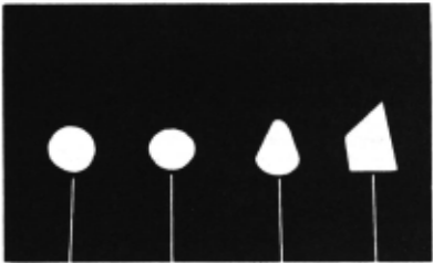
Four objects, as shown in Figure 3, were chosen to determine the system's capabilities with actual images. All four objects were made of wood, finished naturally with varnish. The surfaces were thus visually textured (wood grain) with varying degrees of specularity.
Before normals were computed, a reflectivity deviation map was printed for each object. These maps were examined and a threshold deviation code of 'C' was chosen as the maximum deviation allowable for all cases. From these maps, four high deviation areas were identified on the sphere and spheroid surfaces. These area·s result from specular reflections from each of the sources. On the other hand, the truncated cone and pyramid show specularity only along the edge points. This is as was expected, for the surfaces of these objects were not inc! ined at the proper angle for specular reflection.
The plotted results for each object can be seen in Figures 4 through]. Theses plots show how the essential characteristics of each surface were preserved; each object can be readily
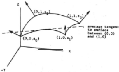
Figure 3. Sample objects for experiment:
- (a) sphere;
- (b) oblate speroid;
- (c) trunca ted cone;
- (d) square pyramid.
identified. This achieved the fundamental objective of this experiment .
On the plotted surfaces of the sphere and spheroid. valleys or dips are visible. These dips are due mainly to the non-uniformity of the I ight source. That is, a flat white disk placed under the scanner did not register a constant intensity at alI points. These surface irregularities are not sufficient to cause the surfaces to be unrecognizable .
The sphere and sphero id surfaces do show profile differences when overlayed, the spheroid being more squat. There was not enough intensity information near the horizon, however, to generate the portions of these surfaces where they differ the most.
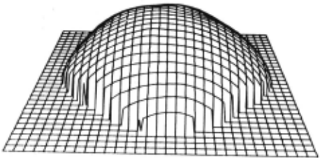
The cone and pyramid gave excellent results . Of particular interest is edge definition and uniformity on the faces. AI I planar surfaces have distinct edges and constant surface orientations . Algorithms, using interpolation or iteration, tend to round these edges and hence are best suited to smoothly curved surfaces.
Profile comparisons between actual objects and the generated surfaces indicated the plotted surfaces were somewhat squat. It is felt that this effect resulted because the camera distance was not large enough with respect to object size. The perspective projection of the imaging device was thus too pronounced to effectively be approximated by an orthographic projection . In all cases, however, the results were very promising and demonstrated the method's abi I ity to handle visually textured, specular objects.
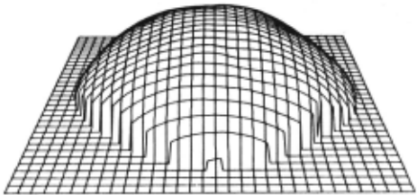
Figure 5. Ohlate spheroid plotted results . Sur face generated from meas ured intensity values. Viewpoint coordinates: (5,-15, 15).
IV CONCLUSION
In this paper ;; have attempted to contribute to the evolution of the photometric approach for surface shape determination in presence of texture and specularity. As a measure of its effectiveness, the results of this approach are most encouraging. It is hoped that this paper wi 11 prove useful in helping to apply shape from shading to surfaces previously thought to be beyond the scope of photometric methods.
@inproceedings{ijcai1981p122,
  title     = {Shape from Shading for Surfaces with Texture and Specularity},
  author    = {Jr., E. North Coleman and Jain, Ramesh C.},
  booktitle = {Proceedings of the Seventh International Joint Conference on
               Artificial Intelligence, {IJCAI-81}},
  publisher = {International Joint Conferences on Artificial Intelligence},
  editor    = {Patrick J. Hayes},
  pages     = {652--656},
  year      = {1981},
  month     = {8},
  note      = {Vision: 3-d},
  url       = {https://ijcai.org/proceedings/1981/122},
}
TY - CPAPER TI - Shape from Shading for Surfaces with Texture and Specularity AU - Jr., E. North Coleman AU - Jain, Ramesh C. T2 - Proceedings of the Seventh International Joint Conference on Artificial Intelligence, IJCAI-81 PB - International Joint Conferences on Artificial Intelligence PY - 1981 SP - 652 EP - 656 UR - https://ijcai.org/proceedings/1981/122 ER -Copied
Machine-readable versions of this paper, for tools and AI agents:
 Welcome
 Future Conferences
 AI Journal Division
 IJCAI Proceedings
 About IJCAI
 IJCAI Awards