Computing Optic Flow

1. Computing~ Flow Cues

1.1 Image Gradient Methods

Fennema and Thompson, and Horn and Schunck derive a computation for optic flow cues based on the assumption of constant brightness (in time) of an object's image [2,4]. If the dynamic image is represented as a scalar field I(x,y , t), then they give the magnitude of the component of optic flow _ in the direction of the (2-D) brightness grad i ent (Ix,Iy) as

where <Ix,Iy,It) is the gradient of I(x,y,t). This computation also assumes that the brightness i s smoothly varying in X and Y. This requi rement i s violated when the local detection window contains any one of the following:

1. An occlusion boundary between objects w1 th different velocities
2. A shadow boundary with a velocity different from that of the shadowed object
3. A specular reflection (highlight) on an object moving relative to that obj ect

All of these cases involve moving boundar i es. It is proposed here that the detection of the motion cues at these boundaries must be computed with respect to some edge operator. 3D-edge operators are interesting in that they provide both the edge and the motion cue information.

1.2 Analysis of Dynamic Images in 3D XYT space

Discontinuities (edges) in the image result f r om discontinuities in the imaging factor s , eg . occlusion of objects, shadowing (occlusion of 1 ighting) , sur face markings , and internal edges of objects (see Table 1).

Table

Imaging factor-- - sur face range sur face orientation incident lighting sur face reflectance Discontinuity occlusion boundary internal object edge shadow boundary surface markings In a dynamic imaging situation we have an image I(x,y,t) with objects that can move, spin, shrink, expand, and deform (translate, rotate, scale, etc.) relative to the camera. Discontinuities in I(x,y,t) can be viewed as two-dimensional surfaces swept out by the edges in successive time-slices of I(x,y,t). These 3D-edges contain information about both the location of 2D-edges in a single frame and the velocity of these edges.

1. 3 Moving 2D-edges as 3D-edges

A small local piece of a 2D-edge is essentially linear and a small local piece of a 3D-edge is essentially planar. Hereafter "2D-edge" and "3D-edge" will refer specifically to these small local pieces. A 20-edge is the intersection of a 3D-edge with an XY plane (a plane of constant T). Conversely, successive occurrences of a 2D-edge sweep out a 3D-edge. The direction (orientation) of the 2D-edge in the XY plane and its velocity determine the orientation of the 3D-edge.

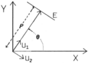
Let a 2D-edge E be represented in polar coordinates ( p,8) as in Fig. 1. In the XYT coordinate system this normal form defines the "static" unit vectors U1 = (cos(8) ,sin(8) ,0) and U2 = (sin( B) ,-cos(8) ,0) in the XY plane which are perpendicular and parallel to E respectively.

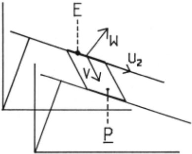
Let the velocity of E be the vector V = (Vx,Vy,1) = d/dt(x,y,t). The 3D-edge P swept out by E moving with velocity Vis parallel to the vectors u 2 and V (see Fig. 2). Thus it is perpendicular to their cross product w = v X u2 = (cos(8) ,sin(8),-Vx*cos(8)-Vy*sin(8) ). This vector defines the orientation of P. Note tha·t the t canponent of W is -<V ,U1>. The inner product <V ,U1> is the length of the projection of V onto U 1.

If we are given P = (Px,Py,Pt) a vector perpendi cular to the 3D-edge P, it must be a multiple of W, viz. p · P = W. -By noting that the projection of W into the XY plane is equal to u1, a unit vector, we see that p = 1/yCPx2 + py2). We then have -<V,U1> = p*Pt, from which we get This is the magnitude of the canponent of the velocity of the 2D-edge per pend icul ar to that edge.

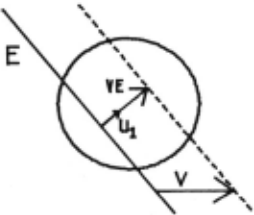
The canponent of velocity parallel to the 2D edge cannot be computed from the 3D edge. This local ambiguity in the detection of optic flow can be demonstrated geometrically in the XY plane (see Fig. 3 from [8)).

The geometric interpretation of local ambiguity in three dimensional XYT space is seen in the fact that the locus of velocity vectors V that would generate P (along with a given u 2 ) is the intersection of P with the plane t = 1 This is a line of solutions so one degree of freedom remains to be speci fled.

2. Computing ~ Flow

2. 1 The velocity vector .!.:! ! pseudo-inter section

An optic now cue provides only one canponent VE of the velocity V of a 20-edge. The actual velocity can lie anywhere on the line in velocity space which has VE as its base vector (see Fig. 4a). This line will be called the velocity line of VE. If we have two non-parallel optic now cues VE 1 and VE 2 for the same actual optic flow, then the intersection of their velocity lines yields a unique solution for the actual velocity (Fig. 4b).

When more than two cues are given for a single velocity, the velocity lines form a bundle through the actual velocity point. In practical applications these lines cannot be expected to intersect at a unique point. Imaging errors, discrete sampling, various noise sources, etc.

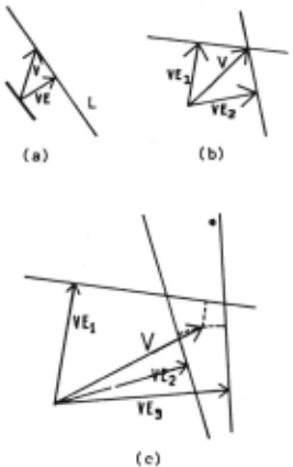
• Figure~_;_ Computing optic now .!E. velocity~ All vectors shown have their tails at the origin in velocity space.
• a)The optic flow V associated with an optic flow cue VE can be any vector lying along the velocity 1 ine L.
• b)Two non-parallel optic flow cues determine a unique flow velocity.
• c)The pseudo-intersection of velocity lines provides a "best fit" flow velocity V for a set of non-parallel optic flow cues VE1.

Figure 2·

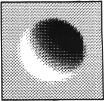
• a)First frame of the translating sphere.
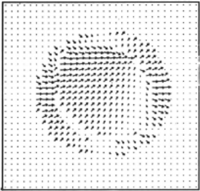
• b)Optic flow cues canputed fran equation 1. 1
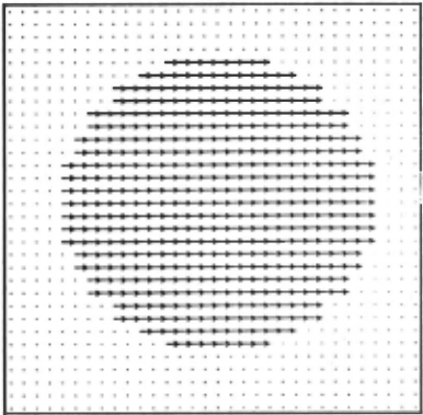
• (')Optic flow derived fran (b) by canputing the pseudo-intersection of velocity lines in local 3 by 3 neighborhoods.

:I .,

~ I

.,

!

introduce alterations in the data and produce errorful measurements of the various VE 1 . Given the measured velocity lines we can look for the point in velocity space that best "fits" these 1 ines. This is the dual problem to that of best fitting a set of points by a line. As in that problem, there are different ways of specifying what is "best". Such measures are typically some function of the distances between the point(s) and the line(s). We have used the least square error (LSE) as the goodness-of-fit measure in our experiments. It reflects a standard intuitive definition of "best fit" and is easy to canpute. The solution for the LSE error fit of a point to a set of 1 ines in a plane is given in [3). This point is called the pseudO-intersection of the given set of 1 ines. Fig. 4c presents an example of the pseudO-intersection of a set of velocity lines.

An application of the pseudO-intersection method (PIM) to optic flow cues. in an image plane is shown in Fig. 5. The first of two artificially generated images of a sphere is shown in 5(a). In the second frame (not shown) the sphere is translated one pixel to the right. The initial optic flow cues canputed fran (1.1) are shown in <;(b). In 5(c) we see the result of t"king the pseudO-intersection of the velocity lines in all 3 by 3 neiRhhorhoods.

Successful canputation of optic flow as the pseudO-intersection of velocity lines depends on those lines being derived fran a single velocity. If optic flow cues fran other velocities are introduced to the ccmputation, the pseudO-intersection is moved towards those velocities and the LSE error increases. This condition may be detected by its high error, but the offending cues cannot be isolated by the

methods discussed so far.

The crux of the problem is the need to partition optic flow cues into sets whose members are all derived fran the sarr.e velocity. In the plane of velocities an equivalent problem can be formulated. There we want to partition the velocity lines into bundles. In the ideal case of errorless optic flow cues and exact velocity lines this problem is easy to solve. In the practical case we must look for good pseudO-bundles, i.e. sets of lines and their solution to this problem has been worked out by Kender [5] who was looking for the vanishing points

pseudO-intersections having low fitting errors. A of texture patt~rns in 2D images.

3. Discussion, Conclusions, and ~ Directions

New approaches have been presented here for the detection of optic flow cues and the canputation of optic flow fran these cues. These two stages operate independently and so can be integrated with the alternative methods of Prager, Fennema and Thompson, Marr, or Horn [3].

The need for detection of moving edges is pointed out and the ccmputation of optic flow at these edges frcm 3D-edges in XYT space is derived. A single step (non-iterative) local procedure is given for ccmputing the optic flow for a set of optic· flow cues.

Related research [ 3] not reported here includes:

1. study of the relevance of particular methods of 3D-edge detection for flow detection;
2. measures of certainty (of results) in the ccmputation of flow b) the pseudO-inter section method ( PIM);
3. iterative flow canputations derived frcm the PIH which are more noise resistant.

Future directions include:

1. study of 3D-edge detection methods that are separable in XY vs. T coordinates (These methods avoid excessive storage requirements):
2. decoupling of local methods of optic flow canputation across edges of discontinuity in flow;
3. integration of slow, iterative, noise resistant flow ccmputation methods [4,8] with the fast PIM.

ACIDICYWLEOOEHENT

This research was supported in part by the National Science Foundation under Grant HCS79-18209. The author acknowledges support frcm a University of Massachusetts Fellowship. The author would like to thank Al Hanson and Ed Riseman for providing

useful ccmments and criticism.