On Shapes

1. Introduction

ON SHAPES

Dana H. Ballard and Daniel Sabbah

University of Rochester Rochester, N.Y. 14627

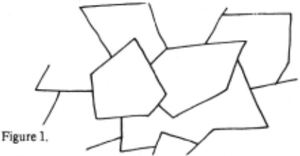
Regions are bounded by linear edge segments which represent the boundaries between planes of different orientation. It might seem a demanding requirement to process image data into the form shown by Figure 1; however, this type of description is easy to compute from range data [Sugihara, 1979] and can also be computed wh_en the surfaces have well-behaved reflectance properties [Ikeuchi, 1980] or once an image has been processed to line­ drawing form [Kanade, 1979]. Thus it seems plausible to assume planar components as input.

An important task in computer v1s1on is to locate a given rigid, 3-d object. This paper describes a representation for rigid 3-d objects together with a Hough algorithm which allows for the detection of such objects from intrinsic image data. Since a description of each object is available, it is detected by finding changes in orientation, translation, and scale of the object from the canonical description.

A central concept of the method is the object·centered coordinate frame. Certain frames seem natural for given objects. For example, a cube is most naturally described with a coordinate frame aligned with its edges. However, there are other choices; one places an axis along the cube's longest diagonal. Experiments with humans have shown that the assignments of such systems can be made dynamically and that different choices often influence _the questions that can he easily answered about the ObJect [Hinton, 1979].

The general object recognition task can be thought of as building a description of the object that has two parts: (l) the description of the object itself (with res~ect to an object-centered frame); and (2) the transfor~ation of the object-centered frame to the viewer-centered (1mage) frame. The reason for this decomposition is parsimony: differe_nt views of the object should have minim~ impact o~ ~~ decription. This is achieved by factormg t~e _obJ~ct s description into two sets of parameters, one wh1ch IS view­ independent (the object-c~nte.red componen_t) and one which is view-varying (the v1ewmg transformation). Often a description of the object is kn~wn beforehand ~nd the task reduces to finding the object-frame to v1ewer-fra!fle transformation. This paper describes a method for handling this case.

The methodology assumes that the image has be~n segmented into planar components such as that shown tn Figure 1. In the image, the planar component correspo~ds to a region of pixels, each of which corresponds to. a P?tnt in the world which has the same surface normal chrection.

The representation descnbes a rigid object with respect to an object-centered coordinate frame. Since the object description is known, the task of determining if the object is in an image can be posed as:

Is there a transformation of a subset of image features such that the subset can be explained as the transformed object?

If the answer to this question is no, then the object is not present. If yes, then the transformation provides all th_e necessary information about the object. It turns out that thts transformation is completely specified by seven parameters: three for translation; three for orientation; and one for scale. This paper assumes orthographic projection, so z cannot be determined, leaving six parameters. The principal feature of our method is that it decouples the interdependence of these three groups of parameters. In other words the orientation of the object can be detected without kno'wing its translation. In fact, there is a natural dominance of parameters:

scale >orientation >translation

The algorithm used is a form of Hough transform usi~g constraint tables [Ballard, 1981]. Image features constram the values for the transform parameters. Each image feature maps only a set of allowable parameter values. When all the features are taken into account, the mapping is many-to-one onto plausible parameter values. Since the cost of this method is exponential in the number of parameters considered together, the decoupling of parameters mentioned before is very significant [Ballard, 1981].

The outline of the rest of the presentation is as follows. First we describe the location of a shape in 2-d, when scale and orientation are fixed. Then we describe how to detect the orientation of the shape without knowing its location. The method for orientation is then extended to 3-d. Finally, we show how the general, 3-d problem can be decomposed into a 3-d orientation problem with a set of 2-d location problems.

2. Representation

In representing shapes, one must keep in mind four different coordinate systems:

1. a two-dimensional coordinate system within which planar surfaces of an object are described (xp.Yp)
2. a three-dimensional coordinate system (xb,Yb,zb) which is an object-centered system
3. a three-dimensional viewer-centered coordinate system (xv.Yv,zv) which describes the environment being imaged
4. an image coordinate system (Xi.Yi) which describes how the world is projected onto a retina.

Assuming orthographic projection, xi = xv and Yi = Yv· The transformation T pb is a known transformation that must be described. Tbv is a transformation which one would like to discover given image data.

2.1 Two-Dimensional Translation

In the 2-d problem assume a shape of fixed orientation and scale. The representation describes the shape as a set of pairs of vectors ((e1·'1),(e2·'2), ... ,(en·'n»· 1be first element of the set, ei, is a directed edge of the boundary of the shape; that is, following ei, ei + 1· etc., traverses the boundary of the object (see Figure 2).

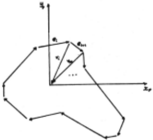
Each 'i denotes a vector from the head of ei to the origin of an object-centered coordinate frame. The representation is redundant since 'i - ei + 1 = 'i + 1 but this redundancy is necessary for the parallel algorithms described in Section 3.

Each ei is represented as an angular orientation and a length (ei,li). 'i is represented as an offset (dx,dy). Ordered pairs (ei·'i) form a translation offset table indexed by ei.

For any orientation ei one can quickly find the offset vi which specifies the position of the body-centered origin.

2.2 Two·Dimensional Orientation

In the plane the angular orientation of a shape is specified by a 'single parameter 0 which denotes the rotation of the body-centered frame with respect to the viewer-centered frame. The representation encodes the orientation i of each edge ei with respect to the bodycentered frame. That way, given an edge oi from an arbitrarily rotated shape which is rotated Om from world coordinates we can compute the rotation of the local frame as am - ai .

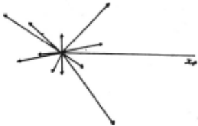
The orientation offsets ei are sorted by length li and form a two-dimensional rotation-offset table of (li,ai) index-value pairs. Figure 3 is a graphical display of this data where the ei pairs are plotted as vectors emanating from the origin. The plot is a 2-d extended Gaussian map [Smith, 1979; Rajcsy, 1980].

Figure 3.

2.3 Three-Dimensional Orientation

In three dimensions, surface areas and surface normals are analogous to edge lengths and edge orientations. The 3d orientation representation is a form of extended gaussian map. Imagine an object with smooth surfaces where a surface unit normal vector is computed for each small value of unit area. The gaussian map is the histogram of such normals, plotted in spherical coordinates. The representation, termed an orientation map, has two important features which incorporate earlier ideas from [Horn, 1980; Smith, 1979; llajcsy, 1980].

First, the representation is explicitly defined with respect to a body-centered coordinate frame whereas the gaussian map is usually defined with respect to a world coordinate frame. In other words, if the object is rotated with respect ot the world, the gaussian map also rotates, but our orientation map does not. Second, there is a hierarchy of structure. The imaged surface of the object is assumed to be segmented into components which are locally smooth surfaces. Each component surface is represented in the orientation map as a single orientation vector together with an associated surface area.

The specific form of orientation map is a spherical coordinate system for orientation, and sorting by area. An object is a set of equal-area surfaces

The above notation means that there are ki surfaces in the set with area Aj- Furthermore Aj > Aj + 1 , 15, j 5, n-1. Both aij and Pij are direction-cosines which describe the orientation of the ijth surface. In the model representation, the direction cosines are measured with respect to the body­ centered frame. In the input data, the direction cosines are measured with respect to the viewer-centered frame.

3. Algorithms

3.1 Detecting Translation in 2-D

In this case the reference origin coordinates (x 0 yc) are the only parameters (rememb~r. rotation and scaling have been fixed). Thus if an edge point (x,y) in an image with gradient orientation e and length I is part of the shape, its reference origin must be at

This constraint is incorporated into a generalized Hough algorithm as follows:

Algorithm A1: Generalized Hough for Shape

Step 0. Make a table for the shape to be located like

Step 1. Form an acc1,1mulator array of possible reference points A(Xcmin:Xcmax .. Ycmin=Ycmax>

Step 2. For each edge point do the following:

Step 2.2a. Calculate the possible centers, i.e., foreach table entry i for e such that

e = ei and I = li compute

Step 2.2b. Increment the accumulator array

Translation that shown in Figure 2. initialized to zero. Step 2.1. Compute e,l(x) Xc := x+~xi Yc := y+~Yi A(Xc.Yc) : = A(xc,yJ+ 1

Step 3. Possible locations for the shape are given by maxima in the array A.

The results of using this transform to detect a shape appear in Ballard[l979].

3.2 Detecting 2-d Orientation

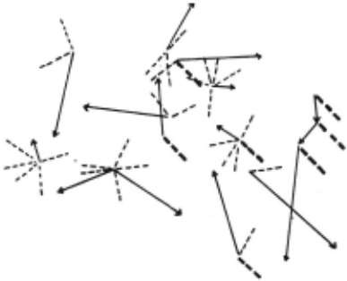
First consider the problem of detecting a rotated two­ dimensional object of known scale. As a simple example, take the shape shown in Figure 2, which appears together with random, directed line segments ifl F;3+.

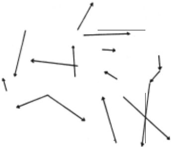
Now for the shape define an intrinsic coordinate system. Then an orientation transform is defined as the following table: for each edge of the sh~p~ m~asure t.he angle required to rotate the edge such that 1t IS aligned w1th the intrinsic x-axis. Figure 5 shows this for the shape.

This graphical example can be expressed formally as the following Hough technique:

Algorithm A2: Orientation Detection

Step 0. Form an Accumulator array of possible orientations A(0 .. 2, ).

Step 1. Foreach edge oriented at angle a, assume its part of the shape and compute the shape's three possible orientations p as

and increment the appropriate accumulator array address

A{ft) : = A{p) + 1 Step 2. Maxima in A correspond to possible orientations for the shape.

If the orientation of the edges in the original "image" was random, the shape should stand out as a particular value of p. However, there is a potential problem with the method: the edges need not be touching each other's end points or even be anywhere near each other to be detected as a shape by the Hough technique. This problem is handled by examining the appropriate edges in the image domain by a kind of reverse Hough transform. Once we have detected a maximum in the accumulator array p· we can eliminate all edges in the image which did not contribute to this maximum. Thus only edges whose orientation a = 0i + p· (where Di is a table entry) are kept.

This pruning can be a parallel process if the edges are stored in a binary array E(x,y,a) where

Once the edge space has been pruned, isolated edges are eliminated leaving only groups of proximal, correctly oriented edges. This does not mean that each group is the shape, since a class of correctly oriented edges but which may be translated with respect to each other are detected by the algorithm. Figure 6 shows some examples of these.

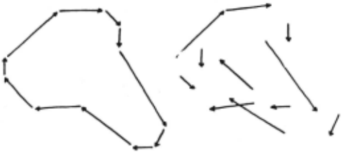
However, the correct shapes can be distinguished from these other shapes by Algorithm A1 once the orientation is known. The key difference between this method and [Ballard, 1981] is that much less space is required· since the parameters are detected sequentially. Only a small array of N6 entries is required to detect orientation and another small array of Nx intrinsic origin locations is required to distinguish the triangular shape. The second array is smaller than the similar array required by [Ballard, 1981] since the reverse transformation localizes the possible origin locations.

3.3 Scale Changes

The method of the previous section can be extended to deal with scale. In this case we can change the table in Section 3.2 to record the relative length of each edge with respect to a standard intrinsic length. Now for each entry we record a ($cale,orientation) pair where the scale is the difference in length of the edge from the reference and the orientation angle is as before. Now scale can be handled in the same way as was orientation. This is shown by the following algorithm.

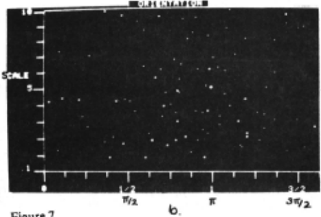
Algorithm A3: Scale and Orientation Detection Step 0. Form an Accumulator array of possible orientations and scale factors A(0:2w . .Smin: Smax>· Step 1. Foreach edge (l,a) and foreach triangle edge ek, compute the orientation p as {I : = a + 0(k) and compute the scale S as s : = 1/l(k) then increment the appropriate accumulator address A{{l,s) : = A(p,s) + 1 . Step 2. Maxima in the Array A correspond to instances of the shape.

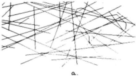
Results of using this transform on an image of directed line segments are shown in Fig. 7. Figure 7a shows the example of Figure 4 which has bee'n rotated by 180° and scaled by a factor of five. Figure 7b shows A {{I ,s).

3.4 Detecting Orientation in 3·0

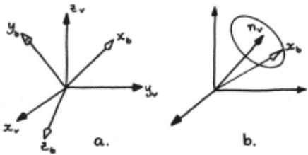
Detecting 3-d orientation is more difficult than 2-d orientation. This is because, given a single surface normal, one can only ascertain the orientation of the body-centered fr8J!le "Yith respect t? the normal. The frame may still be arbJtrarJiy rotated w1th respect to that normal (see Figure 8); however, given a set of planes at different orientations, one can determine the final orientation parameter as the intersection of the loci of the individual normals.

Let uconsider how the surface orientation constrains the object-centered frame orientation. Since the constraint is exploited in a subtle manner we develop it in stages. First, we examine the form of the basic constraint on the intrinsic frame given a surface normal in the viewer·centered frame. Next we show how this constraint could be implemented in general. Finally we show a short-cut that uses the matching normal in the body-centered frame.

Figure Sa and b summarizes the problem for a single normal. Given a normal, nv in the viewer-centered frame (xv - Yv - zv}, the problem is to determine the orientation of the object-centered frame (xb - Yb - zb)· Figure Sa shows this case. Although the object-centered frame must in fact be at a specific orientation, this orientation cannot be determined from a single normal. Instead a single normal constrains the frame to be rotated about the normal at some arbitrary angle. Figure Sb shows this for the xb-axis.

FigureS.

While each individual normal only constrains the frame to a given locus, the frame loci of several distinct normals will be different, and will intersect at an orientation that is correct for the body-centered frame. This orientation can be specified by three parameters. Arbitrarily we use two direction cosines that specify the xb axis orientation and one direction cosine that specifies the x-projection of the Yb axis. Once these are known the rest can be determined from the constraints that the vectors are unit vectors and form a right-handed cartesian frame. That is, where

and ax and Px are known,

Yb is given by (ay. Py. ry) where

and

Finally, zb is determined from

The three components ax, fix· and ay are determined by a Hough technique. Each match between a normal nv and a normal "b determines a locus for a particular set of {ax, fix, ay}. The algorithm is outlined as follows: Let H(ax, f1y· ay) be the number of normals for which the location (ax, Px· ay) of the body-centered frame satisfies the fundamental constraint. The array H is initialized to zero and is generated by:

Foreach match between nv and nb increment all H(ax, fix· ay) where axfJxay is on the appropnate locus.

The maximum in the array H corresponds to the orientation of the body-centered frame.

How can one determine the set {ax, Px· ay} for a particular match? If one possible orientation of the body­ centered frame is known a standard technique for generating the other orientations is to: {l} rotate nv and (xbybzb) so that "v is aligned with an axis (say zv): (2) rotate the resultant XbYbZb about zv: and (3) rotate "v and the rotated (XbYbZb) SO that nv is aligned with its original direction (Fig. 9).

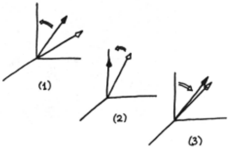
Figure 9.

A short-cut can be taken that takes advantage of the following fact:

If the normal "b· along with (xbYbzb), is rotated so that "b is aligned with the zb axis, then the rotated xbYbzb lie on the appropriate locus.

In other words, the steps in the algorithm that determine the set {axPxry} corresponding to a match between "b and nv are as follows:

• (l) rotate XbYbZb so that "b is aligned wi1h 1.b (the coordinates of nb specify this rotation);
• rotate the result around zv (this generates points on the locus);
• rotate the result of step (2) so that "b is aligned with "v (the coordinates of "v specify this rotation).

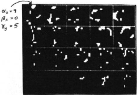
figure 10 shows the results of a simple test of the algorithm. An object with four facets was generated and converted to our surface normal encoding. Next this object was rotated about the z-axis by 30 degrees and this data was used as input. The grain of the array H is -10 units to +9 units. Figure 10 shows this array, mapping three dimensions onto two. The boxes represent successive planes through 1-1 with different values of ay. Within the boxes the different values for H(ax, flx· Yy) are shown. The maximum is at ax = 9, Px = 0, Yy = 5, as expected. The above algorithm assumes scale is known, but can be modified to use the method of Algorithm A3 to deal with unknown scale.

3.6 Detecting 3-d Rigid Hodies

Three-dimensional rigid bodies can be detected by first detecting the orientation of the body. Once the orientation of the body-centered coordinate frame is known it is only necessary to see if the oriented faces have the correct shape. Furthermore this check can be accomplished by a two­ dimensional Hough transform using the representation described in Section 3.1. Thus the five-parameter 3-d problem can be decomposed into a three-parameter orientation problem followed by a two-parameter translation problem.

Initially the representation is augmented by one more parameter whit:h allows the complete specification of the transformation from planar coordinates (xp.Yp) to bodycentered coordinates (xb,Yb,zb).

This final parameter is a rotation w about the out-ofplane axis Zp· This specifies a transformation Tpb which transforms the coordinates of a planar face into the correct position with respect to the body-centered frame. The orientation representation already includes an area and two angles (A, a, b) for each face . Now append w so that the representation for each face is {A, a, h, w). The solution to the face translation problem is to transform the planar shape into the viewer-centered frame by

and then apply Algorithm A 1 to find the appropriate xw.Yw translation.

4. Discussion

The principal result of this paper is to extend the method of [Ballard, 1981] to 3-d. Three dimensions arc harder than two as the number of parameters to describe a shape transformation is seven instead of four. This paper showed : (1) how the Hough technique could be applied sequentially to detect groups of parameters; and (2) how to derive constraint.s within these groups. The methodology is attractive as it can be implemen~ed in parallel, connection­ based architectures [Feldman, 1981; Feldman and Ballard, 1981].

neferences

llajcsy, R. "Three-dimensional scene analysis," Proc., 5th IJCPR, Miami, December 1980.

Aallard, D.H., "Generalizing the Hough Transform to detect arbitrary shapes," TR 55, Computer Sc1ence Dept., U. Rochester, 1979; Pattern Recognition 13, 2, 111-122, 1981.

Ballard, D.H., "Parameter networks: Towaru a theory of low-level vision," TR 75, Computer Science Dept., U. Rochester, April 1981.

Feldman, J.A .. "A connectionist moue! of visual memory," in G.E. Hinton and J.A. Anderson (Eds). Pwallel Models of Associative Memory. Hillsuale, NJ : Lawrence Erlbaum Associates, Publishers, 1981.

Feldman, J.A. and D.H. Ballard, "Computing with connections," TR72, Computer Science Dept, U. Rochester, 19!!1.

Hinton, G., "Some demonstrations of the effects of structural descriptions in mental imagery," Cognitive Science 3, 1979.

Horn, B.K.P. and B.G. Schunck, "Determining optical flow," M.I.T. AI Memo 572, April 1980.

lkeuchi, K., "Numerical shape from shading and occluding contours in a single view," M.I.T. AI Memo 566, February 1980.

Kanade, T., "Recovery of the three-dimensional shape of an object from a single view," TR CS-79-1 SJ, Computer Science Dept., Carnegie-Mellon U., October 1979.

Marr, D. and T. Poggio, "A theory of human stereo vision," M.I.T. AI Memo 451, November 1977.

Smith, D., "Using enhanced spherical images," M.I.T. AI Memo SJO, May 1979.

Sugihara, K., "Range data analysis guided hy a junction dictionary," Artificial Intelligence 12, 1979.