Recognition of 3-D Objects Using the Extended Gaussian Image

ABSTRACT

We propose to use an extended Gaussian image (EGI) for interpreting 2-1/2-D representations for recognition of 3-D objects. The EGI is constructed by mapping each surface normals of an object to the Gaussian sphere.

The freedom in viewer directions caused by incomplete observation is greatly reduced by applying constraints derived from a global distribution of surface normals on the EGI. One constraint on the viewer direction is derived from the ratio of the projected area to the original surface area. The other constraint co~es from the direction of the principal axis. After reducing the possible viewing directions with these constraints, we will apply a matching function to ESis of a candidate set for a final decision.

RECOGNITION OF 3-D OBJECTS USING THE EXTENDED GAUSSIAN IMAGE

Katsushi Ikeuchi

Computer Vision Section Electrotechnical Laboratory Ume zono-1-1-4, Sakura-mura Niihari-gun, Ibaraki, 305 J apan

a global description based on the object-centered coordinate system such as the generalized cylinder (7,8] or the spi ke ~odel [1]. Each local representation depicted as a needle in the above example is obtained at a particular point expressed in viewer-centered coordinate system on the image plane. On the other hand, an object model is expressed in a particular coordinate system usually based on an object cent er and natural axis of the object. These two coordinate systems a r c independent each other. It is quite difficult to recover the original object-centered coordinate system from the 2-1/2-D representation observed in the viewer-centered coordinate system. We propose to use the extended Gaussian i~age (EGI) as a tool for this conversion process·

We also propose an algorithm for reconstruction of the original shape of a convex polyhedron from its EGI. This algorithm is based on the analysis-by-synthesis method.

I WHAT .![ THE EXTENDED GAUSSIAN IMAGE

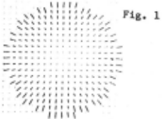
A collection of local surface normals [1,2,3,4,5], sometimes referred to as a 2-1/2-D representation of an object (6], is often provided by machine vision at the low level. For example, an ·algorithm based on the propagation-of-constraints technique [2) provides local surface orientation from shading and occluding infor~ation. The sa~e algorithm can also produce surface orientation from apparent distortion of known patterns based on a regular-pattern gradient map [4]. The distortion of these small circles on the golf ball i n Fig. 1 can be used to recover local surface orientation.

In the above cases, the next problem encountered is how to interpret these local representations for a global recognition of an object. One of the most important issues in this process is how to convert a local representation based on the viewer-centered coordinate system into An EGI of an object may be derived from a spike mode l of the object (1] . A spike mode l is a collection of surface normals on each surface patch in the 3-D world. Let us assume that there is a fixed number of surface patches per unit surface area and that a unit no~al is erected on each patch. The collection of these normals is called a spike model of the object. These normals are like porcupines's quills [1]. These normals on surface patches in a spike model are moved to a common point of application. The locus of points consisting o f their end points lies on the surface of a unit sphere. This mapping is called the Gauss ~ap; . the unit sphere is called the Gaussian sphere. If we attach a unit mass to each end point of the norJqal vector, we will observe a diRtrihution of mass on the Gaussian sphere. This distribution of mass will be normalized. The resulting distribution of mass on the Gaussian sphere is called the extended Gaussian image (EGI) of the object [1,9].

An EGI is independent on both the position of ~he origin and the scale of axes of the coordinate system. A coordinate system may he characterized using three components; the position of origin, the direction of coordinate axes, and a scale factor of a coordinate axis. Among these three components, an extended Gaussian image is independent on both the position of the origin and the scale factor of coordinate axis. An EGI is independent on the position of the origin, because Surface normals on patches will be projected on the Gaussian sphere in parallel transformation without regarding the position of the origin. Also the representation is independent on the scale of the coordinate. For example, a 2x2x2-inches cube has the same representation as a lxlxl inches cube, provided tha t total mass of distribution on the sphere i s normalized. Namely, consist of impulses of pole, the south pole, equator of the Gaussian both images from these cubes 1/6 unit mass at the north and each quarter point on the sphere.

The EGI may be regarded as a unique description, on treating only convex objects. An object has a unique EGI, when the object is a convex polyhedron [10]. Minkowski showed that two convex polyhedra are identical if each pair of corresponding faces has an equal area and the same surface normal.

II RECOGNITION OF AN OBJECT USING AN EGI

A. Data Structure

We have to tessellate the Gaussian sphere into meshes, when we treat objects which have continuous surfaces (eg. cylinder, sphere, ··· ). A continuous surface has a continuous distribution of infinitely many points on the Gaussian sphere. We have to convert a continuous distribution into a discrete distribution.

For tessellation, we have to divide the surface of the Gaussian sphere in ~ uniform ~· Since we look at an object from different directions, a tessellation method is required to have the same resolution of angle in every direction. In other words, each cell on the tessellated sphere is required to have the same area and the same distance from its adjacent cells.

One way to satisfy this condition is to use a regular polyhedron to divide the Gaussian sphere into meshes [11]. A regular polyhedron has faces of equal area. Also a regular polyhedron has faces evenly distributed in direction with respect to the center of gravity. Thus, we can divide a sphere into meshes of a fixed area by projecting edges of a regular polyhedron inscribed in the sphere onto the surface of the sphere with respect to the center of the sphere. The resulting tessellation on the sphere is called as a geodesic dome [12).

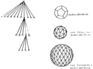
Since we have no polyhedron of higher order than the icosahedron, we use a semi-regular geodesic dome constructed from a two frequency dodecahedron. (See Fig. 2.) Our tessellated sphere also has a hierarchical structure. Each cell on one level contains both pointers to sub-cells on the next level and the direction of the center point of the cell. Distance measures between cells is also maintained in this structure. Since we use a two frequency dodecahedron for tessellation, the top level cell contains pointers to twelve surfaces of a geodesic dome based on a dodecahedron. The second level has 60 triangle areas which come from a one frequency dodecahedron. The lowest level contains 240 triangle cells of a two frequency dodecahedron.

Quantization of an object in all directions uniformly is also required when making a prototype. For example, if you sample surface orientations of an ellipsoid along its long axis at every observed picture element, you will obtain very rough information on the view from the direction of the long axis even though you get fine information on Fig. 2 Data structure. Each cell, depicted as a circle, contains both pointer to sub-cells on the next level and the surface orientation there.

· "''"''

the view from the direction perpendicular to the long axis. Thus, this sampling method is quite unsuitable in this case. We will use the tessellated sphere for sampling directions when making prototypes as well as for registration of the EGI. The tessellated sphere samples the whole spatial directions in an even manner. This schema will give an even sampling with respect to every direction.

Note that two spheres are used; One for sampling spatial directions and the other for registering an EGI on its spherical surface. The former sphere for sampling is assumed to be located at the center of gravity of an object. Surface orientation of patches on an object arc sampled at every direct i on corresponding to each cell on the tessellated sphere. In other words, the surfa~e normal on each cell of the sampling sphere is extended until it reaches the surface of the object. At that surface patch where the extended surface normal hits, surface orientation of the object is measured. The measured surface area will be registered on the correspo~ding cell of tessellated Gaussian sphere for expressing the EGI of the object. Thus, the cumulative image on the sphere for registration is constructed as the EGI for the prototype of the object.

B. Constraints ~ Viewer Directions

Matching an EGI from observed data with its prototype involved three degrees of freedom, since there are three degrees of freedom to altitude of an object in space. If the whole surface of an object was visible, the directions of the three principal moments of inertia would determine the spatial alignment of the object [9). Unfortunately, however, the typical situations allow us only a partial observation of an unknown object. This partial observation causP.s three degrees of freedom in altitude of the object. Viewer direction gives two degrees of freedom; that is, there are two degrees of freedom corresponding to which cell on the Gaussian sphere of a prototype is perpendicular to the direction of the line n1' sight. The remaining degree of freedom comes !."r-om rotation of the Gaussian sphere of the prototype around the line of sight when matching the prototype with the observed sphere.

We will use two kinds of constraints to reduce the search space for matching. Although a brute force technique, such as search through the space of possible attitudes, can be applicable to matching directly, we will reduce this search space using constraints before beginning comparison. One constraint reduces the freedom of viewing direction. This constraint is derived from a ratio of visible area projected onto a plane perpendicular to the line of sight against surface area. The other one constrains freedom of rotation. This constraint for rotation of the sphere is based on the symmetry axis on the plane perpendicular to the line of sight.

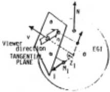
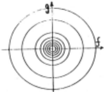
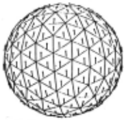
The ratio of area projected onto the image plane against the original surface area is a constraint on the viewing direction. For example, observing an ellipsoid from the direction of the long axis gives a smaller projected area than looking at the same ellipsoid from the direction perpendicular to the axis. Yet the surface area is Fig. 4 The ratio of the Fig. 5 The direction of the same.

Projected area is normalized by surface area. The area is calculated at each triangle v beforerat os are ep cte as seeing t e 0 ject comparison. See Fig. 3. This ratio is denoted as

Av · sum (Zi x Mi) I sum (Mi),

where the summation is done only if the mesh i is visible from the mesh v, Mi is mass at the cell i, and Zi is a inner product between the viewer direction v and the surface normal at the cell i. This ratio is calculated only over a visible hemisphere from the viewing direction v. This ratio removes only one degree of freedom just like the reflectance ratio on the Gaussian sphere [2]. Thus, even though this constraint reduces the possible set of of viewer directions, we still have to search for the real view point on the Gaussian sphere along one of these iso-ratio lines observed from an image. For example, Fig. 4 denotes iso-ratio contours drawn on the stereographic plane for graphical clearness. This diagram is use·d when finding viewer direction in the same way as the reflectance map is used to recover the 2-1/2-D representation from a brightness value.

We also must find the rotation of the EGI of a prototype around each candidate cell for the viewer direction. We use the direction of the principal axis of inertia over a hemisphere from the viewer direction. We will use the 2-D axis rather than the 3-D axis for simplicity of calculation. In other words, we use the direction of the axis of least inertia on the tangential plane at cell v (or the image plane on seeing the object from the direction of v).

The direction cell i is cell v. the plane. following calculation will give the of this axis. Before calculation, each projected onto the tangential plane at the Let (Xi,Yi) be the coordinate obtained on We will use

Ixx Sum( Mix Xi x Xi),

Ixy Sum( Mix Xi x Yi ),

Iy)l' R Sum( Mix Yi x Yi ),

surface area to the principal axis of inertia projected area. These at each image plane on i d i d h b f rom contours on the each direction. The hi 1 The stereograp c p ane. prototype and the observed ratios constrain viewer image should be alingned directions. along this direction.

where these summation are also done only if cell i is visible from the cell. From these values of Ixx,Ixy,Iyy, the principal direction of inertia is obtained.

~ ·(atan(2Ixy/(Iyy-Ixx)))/2,

This~ is the direction of the principal axis on the tangential plane.

This direction may be regarded as a symmetry axis of the object observed from the direction denoted with the cell v. Note that, if the object has a symmetry axis in the 3-D space, the principal direction of inertia in 2-D obtained above will correspond to the direction of 3-D symmetry axis projected onto the plane [9]. In other words, the direction is unique at each cell in almost all case. Thus, this direction uniquely determines the manner in which way a prototype should be aligned on comparing the prototype with an observed data. In this case, the constraint reduces the possible area perfectly; there is no need for search involved. In Fig. 5 the direction of principal axis of inertia at each viewing direction is depicted as a needle on each cell v. These needles constraint the rotation of prototype around the line of sight.

So far each cell on the Gaussian sphere has to contain three kinds of information; how much weight the cell contains (mass), how much an object has projected area on being viewed from the direction of the cell (surface ratio), which way the axis of inertia exists (axis). The second one (surface ratio) and the third one (axis) constrain freedom of viewing direction before matching. The first one

(mass) is used for final decision based on a matching function mentioned in the next section.

C. Matching Function

The following matching function is comparing an EGI obtained from a representation with images of prototypes. used for 2-1/2-D

if M-proto(cell-number) equal 0.0 do nothing if M-proto(cell-number) not equal 0.0 then setq difference (- M-proto(cell-number) distance M-observed(cell-number+e)) (distance cell-number if ( diff and dist then cell-number+e) difference-standard distance-standard) add exp ((- diff x gl)+(- dist x g2)) to total-point

where gl and g2 are coefficients. In other words, if a cell in the prototype has so~e contents, the algorithm checks around the cells in the observed data to see whether the observed data contains similar amounts of mass or not. In case there exists a similar amount of mass within a neighboring area, a weight will be added to the point-total for the prototype. After calculating this point-total for all candidates, the candidate obtaining highest point-total will be determined as the object observed.

D. An Illustrative Example

Consider the simple example of an ellipsoid (~+Y~+(Z/5)&·1) observed from the direction inclined from Z axis by angle 10 degrees. The surface normal will be derived analytically and used to generate a needle diagram. The algorithm will be applied to the synthesized needle diagram. The result will be used as a basic basis for judging the performance of the algorithm.

For the example, a 40 x 40 synthesized needle-diagram was generated. At each image point, e~ementry calculus gave an outer surface normal of the ellipsoid. For graphical clearness, each surface normal is depicted as a needle.

The first task is to obtain an EGI from this needle diagram. Each surface normal at an image point is determined to which cell on the gaussian sphere the surface normal corresponds. Then, its surface area is added to the cell. Since each image point is assumed to have the same area, corresponding surface area is calculated as

(1/ cos<X).

where « is the angle between the surface normal and the direction of the viewer. After obtaining surface areas, cumulative values registered on cells of the Gaussian sphere are normalized by the surface area observed. Fig. 7 showes the resulting EGI obtained from Fig. 6.

We also determine the ratio of the projected area to the surface area, while making the EGI from the needle diagram. This ratio reduces possible viewer directions as mentioned above. The surface area is calculated simply by summing up (1/ cos«), while the projected area is as same as the number of image points within the occluding bound,ary. Strictly sp;ak}ng, we only use the points within a boundary (/f +g < 0.9 ) when obtaining the surface area, because points near the occluding boundary cause a dramatic effect to this value. For example, if a point sits at the occluding boundary, (1/ coson becomes infinite; we cannot obtain the real surface area.

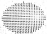
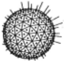
Fortunately, the constraint, the ratio of the projected area to the surface area, also works within some boundary. More precisely, the ratio is a function of both a spatial angle on the gaussian sphere and the viewer direction. For example, if we take into account all points on a hemisphere of the Gaussian sphere, the ratio is the constraint to the viewer direction as the one mentioned above. On the other hand, if we use only points within a cell, the constraint is identical to the judgment whether the cell contains some amount of mass or not. Between these two extremes, we can also derive various kinds of constraints, depending upon which area on the gaussian sphere we use for calculation. In this example, we use the ratio of the projected area to the surface area whose corresponding points on the Gaussian sphere have azimuth an~les less than 85 degrees based on the direction of the viewer ( jf1 ~ ( 0.9 ). We obtained 0.27 as the ratio within the boundary in this illustrative example.

We prepared two kinds of EGis as candidates for matching. One is from the ellipsoid and the other one is from an cylinder whose radius is 1.0 and hight is 1.5. Their EGI is shown in Fig.8.

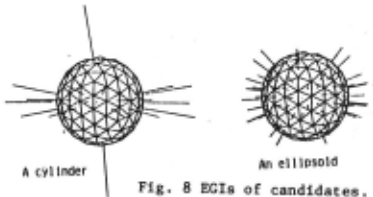
The ratio of the projected area to the surface area (0.27!0.1) reduces 240 possible viewer directions to 21 directions in the case of the ellipsoid and to 43 directions in the case of the cylinder. Since both objects have syrunetry axes, the constraints from the axis determines the direction of alig~ent uniquely.

In the ellipsoid case, cell 16 (and cell 220 the opposite side of 16) has the highest value, 6.59

and cell 0, 8 has the second largest value 6.07. In the cylinder case, cell 0 has the largest value 1.40. Namely, the algorithm tells us that the cell number 16 of the ellipsoid is most likely as the viewer direction. This cell has the direction (0.1426, -0.1036, 0,9843) based on the direction of the long axis' of the ellipsoid. In other words, the algorithm successfully tells us that it is most likely that the ellipsoid is observed from the direction inclined by 10.15 degrees from the long axis of the ellipsoid.

III RECONSTRUCTION ~F A CONVEX POLYHEDRON ~ ITS-EGI

If an object is a convex polyhedron, it is possible to reconstruct the original shape from its EGI. This result can be predicted from Minkowski's theorem [10]. This theorem is quite important. Because of it, we need. not store the adjacency relationships among faces. Only the surface orientation of each face and its area need be remembered. Actually, this fact is the basic motivation for using an extended Gaussian image.

Unfortunately, Minkowski's proof of the theorem is not constructive and does not provide an algorithm for reconstruction. We propose here an algorithm for this reconstructing of a convex polyhedron from its EGI. Our algorithm for reconstruc,ion is based on the analysis-by-synthesis method.

The problem for reconstructing a shape from its EGI is to obtain the distances of the faces (Co, ··· ,Cn) from an origin, provided that we have known areas (Mo, ··· ,Mn) of faces and the surface orientations ((Xo,Yo,Zo), ··· ,(Xn,Yn,Zn)). We may set Co·O without loss of generality, because a polyhedron can be put at an arbitrary place in a part:icutar coordinate system without altering its shape.

We can divide the problem into n cases. There always exists a maximum value C-max among Cl, ·· ,cn. That is, there is a farthest face from the origin among face 1, ··· ·face n. Thus, we will consider n sub problems. Namely, in case i, we assume Ci has the maximum value; face i is the farthest face from the origin. We set the farthest distance, Ci · 1.0, in case i. The reason for dividing the problem into n cases is to fix the possible values of the Ci between 0.0 and 1.0. Otherwise, Ci may take a value from 0.0 through an infinite value. Since we do not know whir.h case is true amonp, the n cases, we will check all n cases to see wheth~r the case contains a solution point or not. For each case, we will quantize the remaining n-2 diMensional space into cells where Cl, ·· ,Ci-l,Ci+l, ··· ,Cn changes from 0 through 1.0. Then, it is possible to calculate Mo, ··· ,Mn at each mesh point (Co, ··· ,Cn) and to compare with the given values.

We will show how to calculate Mo as an illustration. Obviously, another face area Mi can be obtained in the same way.

For simplicity, (O.o,o.o,l.O), where we assume (Xo,Yo,Zo) (Xo,Yo,Zo) denotes the unit normal vector corresponding to the surface orientation of face 0. This can be established by rotating the Gaussian sphere so that the vector (Xo,Yo,Zo) points to the north pole. In other words, (T (Xo,Yo,Zo)) · (O.O,O.O,l.O), where Tis a matrix which corresponds to one of the suitable rotations.

The other points on the Gaussian sphere should also be rotated in the same way;i.e. (T (Xi,Yi,Zi)). In the following part we denote T (Xi,Yi,Zi) by (Xi,Yi,Zi) for the sake of simplicity.

We next determine whether one intersection line constitutes an edge of the face for (Xo,Yo,Zo) or not. Every face corresponding to (Xi,Yi,Zi) has an intersection line with the infinite plane corresponding to (Xo,Yo,Zo). The desired face corresponding to (Xo,Yo,Zo) consists of a partial plane cut out from the infinite plane by some segments of these intersection lines.

Since a face of a convex polyhedron is also convex, the algorithm can connect only those segments which constitute a convex figure. If a small bug is assumed to travel along edges of a convex figure counter-clockwise, the bug would always turn to the left at each corner of the convex figure. In other words, the ~ormal vector from each edge (and also the projection of the surface normal of a face which intersects the infinite plane constituting the edge) also rotates clockwise. For this, we will order the intersection line according to the azimuth angle (atan(Yi/Xi)) of the normal vector (Xi,Yi,Zi) of each face i. (we will denote the n-th intersection line as Ln), then the bug will visit intersection lines in the order sometimes skiping some lines.

We calculate the intersection point between the n-th line and the n+l-th line (we will denote this point Pn,n+l), These points are candidates for vertices on the face of the polyhedron. We will connect Pn-l,n with Pn,n+l, In other words, we will cut out a segment~ between P~,n and Pn,n+l from the intersection line Ln, where Sn has the direction from Pn-l,n to Pn,n+l.

_ We will connect~ from PO,m in sequence. If Sn+l turns around Pn,n+l counter-clockwise based on the direction of the segment~ then the ;egment:s; is an edge of the face, If ~ turns around Pn n+l clockwise, then sn+\ is not an edge of the face,' We rRll this seroaent ~1 as an imaginary edge and do thde imaginary-edge operation in order to find a real e ge.

The imaginary-edge operation recalculates a segment which causes an imaginary-edge. Let us assume that !f:r is detected as an i~~inary-edge. It means that the last segment S -1 should be also re-calculated, because the ~st s~ent ~ is assumed to intersect with Si but Si is not a real edge. The iMaginary-edge operation will recalculate each intersection point between Li-1 and Lj, where j is larger than i and make a new segment,___jhe imaginary-edge operation will find a segment S'i-1 whose length is smaller than ~1 for the first time after Li along the sequence. (See Fig. 9.) This segment S'i-1 between Pi-2,i-l and Pi-l,j is returned to the main operation as an edge of the face. This imaginary-edge operation is called recursively, if necessary, Fig. 9

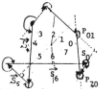
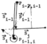
(A) At first, all adjacent (B) An imaginary-edge segments will be connected operation re-calculates a on their azimuth angles, segment which causes an imaginary edge,

After finding all real segments, the face area will be obtained as

where o~. = 'i-..t.u, 4· .. · , ... t.n, 44

.4.; = 'Xi '$,., - 'X ·· , "~ 0-th and i-th plane are denoted as

In the above calculations, i visits only real edges in aequence, After obtaining all areas Mo,.,.,Mn, the areas will be normalized, Comparison with the goal will be done as

where Mk, Mk-proto are areas corresponding to the face (Xk,Yk,Zk),

IV CONCLUDING REMARKS

We proposed the use of the EGI for interpreting 2-1/2-D representations obtained from raw data for recognition of 3-D objects. While a 2-1/2-D representation is based on the viewer-centered coordinate system, a 3-D description is expressed in an object-centered coordinate system, This discrepancy between the two kinds of representations may be overcome by using the EGI, since the extended Gaussian image is essentially independent of the coordinate' system,

Incomplete observations cause freedom in viewer directions and rotations in the space on matching, The freedom is greatly reduced if we apply constraints derived from a global distribution of mass to the matching process. So far each cell contains the mass of an EGI at that point, surface ratio representing how much a surface is projected on a plane perpendicular to a viewing direction, and the direction of a symmetry axis relative to the viewing direction, - After reducing the possible directions of observation, a matching function is applied to the observed distribution of mass with the prototypes of candidates objects, The best fitting candidate will be selected as the object observed at that time, Even though a couple of non-convex objects among a candidate set may have the same F.GI [13], an EGI is still a helpful tool; after reducing the possible set of candidates and also determining possible spatial alignments of the candidates by using the F.GI, the interpreter can make a final decision based on the other features such as position information, which the F.GI discards in order to overcome the discrepancy between the viewer-centered coordinate system and the object-centered coordinate system,

ACKNOWLEDGMENTS

The author would like to extend his sincere appreciation to Dr, Y, Shirai of ETL and Prof, B,K.P, Horn of MIT for their helpful discussions, Thanks go to the referee's to their helpful comments.