
Towards a Mathematical Theory of Program Synthesis
Proceedings of the Sixth International Joint Conference on Artificial Intelligence. .
© 1979 International Joint Conferences on Artificial Intelligence
Abstract
This paper attempts to set a theoretical foundation for Program Synthesis. A programming language Prog is introduced together with its interpretation in the semantic domain D. A formal system QFT, which is an extension of the Heyting arithmetic, is then introduced in order to express specifications formally. Roughly stated, the main result is: Given a QFT-proof of the specification ~x~zA[x,z], it is possible to construct a program p such that A[x,p[x]] is true in D for any input x. Moreover, a formal proof of ~xA[x,p[x]] can also be obtained. Since any program p in Prog always terminates, the above result establishes the total correctness of the synthesized program at the same time. Finally, it is shown that any program p in Prog can be faithfully simulated by means of LISP.
- Burstall, R.M. and Goguen, J.A. 1977] Putting thories together to make specifications, Proc. IJCAI-77. MIT, Cambridge, Mass., 1045-1058.
- G~del, K. 1958] Uber eine bisher noah nicht benUtzte erwriterung des finiten Standpunktes, Dialectica, 12, 280-287.
- Goto, S. 1978] Program synthesis through ~del's interpretation, Proc. International Conference on Mathematical Studies of Information Processing, 287-306, Kyoto.
- Howard, W.A. 1970] Assignment of ordinals to terms of primitive recursive funotionals of finite type, Intuitionism and Proof Theory, 443-458, North-Holland.
- Kreisel, G. 1977] Some uses of proof theory for finding computer programs, Colloque International des Logique, 123-134, Paris.
- Shoenfield, J.R. 1967] Mathematical Logic, Addison Wesley.
- ShUtte, K. 1977] Proof Theory, Springer.
- Takahashi, M. 1977] A foundation of finite math- ematics, Publ. RIMS, Kyoto Univ., 12, 577-708 .
- Takasu, S. 1978] Proofs and programs, Proc. 3rd IBM symposium on Mathematical Foundations of Com- puter Science, IBM Japan.
- Takeuti, G. 1975] Proof Theory, North-Holland.
- Troelstra, A.S. 1972] Review of [Yasugi 1963], J. of Symbolic Logic, 37, 404.
- Troelstra, A.S. 1973]--Mathematical Investiga- tions of intuitionistic arithmetic and analysis, Lecture Notes in Mathematics 344, Springer.
- Yasugi, M. 1963] Intuitionistic analysis and ~del's interpretation, J. Math. Soc. Japan, 15, 101-112.
References were extracted automatically from the PDF and may contain errors.
Full text extracted automatically from the PDF; figures, tables and equations may differ. The PDF is the version of record.
1. FUNCTIONALS OF FINITE TYPE
- ~
Definition of types:
- The symbol 0 is a type.
- If a and T are types then [a~] is a type. For brevity we write a 1 ~ 2 ~ ··· ~n~ instead of
[a 1 ~£a 2 ~ ··· ~[a ~T] ··· ]]. The set of all the types will be aenoted by Type.
1.2 Terms and programs
The terms of FT will be constructed from the following language LFT:
- Denumerably infinite set FVa of free vari ables for each type a: FVa·{ala,a2a,a3a, ··· }. We put FV·u{FVaia£Type}.
- Denumerably infinite set BVa of bound vari ables for each type a: BVa·{xla,x2a,x3a, ··· }. We put BV·u{BVaia£Type}.
- Constants: O(zero), S(successor) and J (iterator) for each type a. a
- Lambda abstraction symbol: A.
- Parentheses: (and ).
As auxiliary symbols, we have denumerably infini tely many nominal symbols: *1,*2,*3, ···· By an n-plaae (LFT) nominal form we mean a finite string of symbols which contains, in addition to the sym bols of LFT, at most the nominal symbols *1,*2, ··· ,*n, where n is the decimal numeral which represents the natural number n. If A is an n-place nominal form and r 1 , .·· ,rn are strings of symbols, then A[r 1 , ··· ,r] aenotes the result of replacing n - every occurrence of *i in A by ri(ls i sn). We will use italic letters to denote nominal forms.
Definition of the set Tm of terms, type: Tm+Type and bvar: Tm+2BV:
1. a£FV => aETm, type[a]=a, bvar(a]=¢,
2. OETm, type[O]=O, bvar[O]=¢.
3. SETm, type[S]=~O, bvar[S]=¢.
4. J €Tm, type[J ]=~[a~]~~o, bvar[J ]·¢.
5. r~ SETm, typefr]=a~T, type[s]=o, bvgr[r]n
bvar[s]=¢ => (r s)ETm, type[(r s)]=T, bvar[(r s)]· bvarfr)ubvar[s].
- r[a]€Tm, type[r[a]]·T, aEFVa, X€BVa-bvar[r[a]] ·> Axr[x]€Tm, type[Axr[x]]·a~T, bvar[Axr[x]]= bvar[r[a] )u{x}.
Tm is the least set which satisfies the above con ditions. We put Tma={t€Tmltype[t]·a}. An element in Tma is called a term of type a. Two terms r and s are congruent if they are constructed exact ly in the same manner, except that possibly dif ferent bound variables are selected in the appli cations of 6 above. We will henceforth identify congruent terms. This identification has the ef fect of making bound variables really dummy . A program is a term containing no free variables. We waite Prog for the set of programs, and we put Prog ·{t€Progltype[t]·a}. We use r, s, t etc. as syntactic symbols denoting terms or programs. For brevity we write r 1 r 2 r 3 ··· rn instead of (( ··· (r 1 r 2 ) r 3 ) ··· ) r ).
Definition ofna binary relation red on Prog:
- (Axr[x] s) red r[s].
2. J Os t red t ·
3. Ja(Sr)st red s(J rst).
4. rared r 1 => (r s~ red (r 1 s).
5. s red s 1 a> (r s) red (r s 1 ).
We let red* be the reflexive and transitive clos ure of red. A program p is normal if p red q for no q.
Definition of the numerals N (n: a natural number): n
1. N 0 ·0.
2, Nn+l·(S Nn).
The following three lemmas can be proved by a standard technique. (See, e.g., [SchUtte 1977], [Troelstra 1973], [Howard 1970].)
Lemma 1. A program p of type 0 is normal if and only if p·Nn for some natural number n.
LeDDDa 2. If p red* q, p red* q 1 , and both q and q 1 are normal, then q·p'.
LeDDDa 3. For any program p there e:r:ists an nor mal program q such that p red* q.
Putting LeDDDa 2 and Lemma 3 together, we have: Theorem 1. For any program p there uniquely e:r:ists an normal program q such that p red* q. The program q in the above theorem is called the normal form of p, and is denoted by [p]. We write D for the set of programs in normal form, and we put Da={pEDitype[p]·a}.
1.3 Interpretation of terms
We can use the function [ ]: Prog+D which sends a program p to its normal form [p], as a semantic function. For instance, a program p of type a~ may be considered as denoting a functional p: Da+DT such that p[s]·((p s)] for any sED 0 · Fur-
0 thermore, we remark that, by Lemma 1, D is isomorphic with the set IN of natural numbers. With this interpretation in mind, we define the formal system FT of primitive recursive func tionals of finite type as follows.
2. THE FORMAL SYSTEM FT
- Definition of the system FT Definition gf the set Form of FT-formu~s: 1. s, tETm => s·tEForm.
- A, BEForm a> (A~B), (AAB), (AVB)EForm. We use r, 6 etc. to denote finite (possibly empty) sequences of formulas. If r is the sequence 1 Al, ··· ,A I then r~B is the abbreviation of Al~ ··· ~A ~B ~ich, in turn, is the abbreviation of (Al~(~ ·· ~(A ~B) ··· )). If r · 1 Al, ··· ,A I and 6· 1 B 1 , ··· ,Bm 1 nthen rs6 means that these~ {A 1 , ·.· ,
A} is included in the set {B 1 , ··· ,B }, We define n m the connective -.by:-,A=A~so-o. A formula con taining no free variable is called a alosed for mula. A formula which .only contains equations be tween terms of type 0 is said to be a basia for mula.
Definition of the provability relation r in FT: Axioms:
(A) r (Axr[x] s)=r[s].
(J 0) ~ J Ost·t.
(=) r s·t~F[s]~F[t]. Inference rules:
(JaS) r Ja(Sr)st·s(J rst). a a a
(Str) r r~B, rs6 ·> r 6~B.
0 (CI) r F[O], r F[a]~F[Sa], aEFV , atF, tETm => I- F[ t].
(Cut) r r~A, r A~B => r r~B. O
- (Al) r A~B~C=> ~ (AAB)~C.
- (Ar) r r~A, r r~B => r r~(AAB).
- (vl) 1- A~C, r B~C => ~ (AvB)~C.
- (vr) ~ r~Ai => r r~(A 1 vA 2 ) (i·l,2).
In the above definition, alF means that the free variable a does not occur in the nominal form F. A formula A is said to be provable (in FT) if rk.
2.2 Consistency and weak completeness
Definition of truth and falsity for a closed for-
- mura:
1. A closed formula s=t is true iff [s]=[t],
2. A closed formula A~B is true iff A is false or B is true.
3. A closed formula AAB is true iff A is true and B is trul3.
4. A closed formula AvB is true iff A is true or B is true.
5. A closed formula A is false iff A is not true. We write ~A if A is true. We then have the fol lowing consistency theorem. (See [SchUtte 1977], Theorem 17.2.)
Theorem 2. ~A. A: alosed => ~A.
Although not all true closed formulas are prov able in FT (example: -.J 0 (SO)S·S), we have the following weak completeness theorem.
Theorem 3. ~A. A: basia => t- A.
Putting Theorem 2 and Theorem 3 together, we have: Theorem 4. A alosed basia formula is provable in FT if and only if it is true.
3. THE FORMAL SYSTEM QFT
3.1 Definition of QFT
Definition of the set Form of QFT-formulas and BV bvar:Form+2 0 :
1. s, tETm ·> s·tEForm, bvar[s·t]·bvar[s]u bvar[t].
2. A, BEForm => (A~B), (AAB), (AAB)EForm, bvar[(A~B)]·bvar[(AAB)]=bvar[(AvB)]·bvar[A]u bvar[B]. a a
3. A[a]EForm, aEFV , xEBV -bvar[A[a]]·> ~[x], ~xA[x]EForm, bvar[YxA[x]]·bvar[3xA[x])·bvar[A[a]] u{x}.
Two formulas are aongruent if they are construct ed exactly in the same manner, except that poss ibly different bound variables are selected in the applications of 3 above. We will henceforth identify congruent formulas. A formula is quan tifier free if it contains no occurrence of ~ or 3. A quantifier free QFT-formula is just a basic FT-formula. We define the negation~A of a for mula A by ~=A~SO=O.
Notational aonventions: Let s· 1 s 1 , ··· ,s 1 be a d 1 1 n I sequence of terms s 1 , ··· sn an et t· t 1 , ··· ,tm be a sequence of terms t 1 , ... ,tm' where m,n~O. Suppose that type[si]·a 1 ··· +crm~i(l~i~n) and type[ti]·Ti(l~j~m), Then we let (s t) denote the sequence 1 s 1 t 1 ··· t , ··· ,s t 1 ··· t 1 , We user, s, t etc. to denote s~quencenof terms. Similarly, we use a, b, c etc. to denote sequences of free variables, and x, y, z etc. to denote sequences of bound variables, If x· 1 x 1 , ··· ,xn 1 ' t· 1 t 1 , ··· ,tn 1 and A is ann-place nominal form, then YXA[x], 3xA[x] and A[t] are the abbreviations of Yx ,,, vxnA[xl'''''xn]' 3xl···3XnA[xl'''''xn] and A[tl' ·.· ,t J, respective y.
Defin~tion of the provability relation ~ in QFT: Axioms:
(FT) r A (in FT), A: basic ·> -A.
('fl) t- '(fxA [x] ~A [ t 1,
(3r) t- A[t]~3xA[x].
- (IPO) A:quantifier free ·> r ~xA[x]~3yB[y))~ 3y(VxA[x]~B[y)).
- (M 1 ) A:quantifier free ·> r~3xA[x]~3xA[x].
- (AC) r~3yA[x,y]~3zVxA[x,zx].
Inference rules
(Str), (Cut), (CI), (Al), (Ar), (vl) (vr): same as in FT for QFT-formulas.
(Vr) 1- r=>A[a], a~A ·> 1- r=>~.xA[x].
(il) 1- A[a]=>B, a~A ·> 1- 3xA[x]=>B.
In the above definition, a~A means that none of the free variables in the sequence a occurrs in the nominal form A. Also in the above definition, IP, M and AC stand for 'independence of premiss', 'Markov's principle' and 'axiom of choice', re spectively. Two formulas A and B are equivalent in QFT if both A=>B and B=>A are provable in QFT.
3.2 Interpreting formulas
A QFT-formula F is an interpreting formula if it is of the form ~xyYF 0 [x,y], and F 0 is quantifier free. (We use the subscript 0 to denote a quan tifier-free nominal form.)
Definition of �~del translation: With each QFT formula F, we associate an interpreting formula F* (~del translation of F) as follows.
- F: ~uantifier free ·> F*·F.
Let A*· x 1 Vy 1 A 0 [x 1 ,y 1 ] and B*·3x 2 Vy 2 B 0 [x 2 ,y 2 ].
- F·A;;B ·> F*·3X 2 3y 1 Vx 1 yy 2 (A 0 [xl'ylxl'y 2 ]=> BO[x2xl'y2]).
3. F·AAB ·> F*·3x 1 3x 2 Vy 1 Vy 2 (A 0 [x 1 ,y 1 JA Bo[x2 ,y ~]).
- F·AVB · F*·3z3x 1 3x 2 Vy 1 Vy 2 (z·O=>A 0 [x ,y ] A,z·O=>B [x y ]) 1 1 0 2' 2 ·
Let (A[a])*·3x 1 Yy 1 A 0 [x 1 ,y 1 ,a]
5. F·YxA[x] · F*·rx Vrty A ['x x, y x].
6. F·3xA[x] · F*·~ 1 vyiA~[xi ,y J:J. The following theorem can be veritied without difficulty. (AC) playa a role in the proof. Theorem 5. For any QFT-formula F, F and F* are equivalent in QFT.
3.3 Reduction of FT to FT
Let F·3x F [x,y) be an interpreting formula. A quantifier ~ree formula F 0 [t,a] is called a re duction of F, if a is a sequence of free vari ables such that a~F 0 , and if t is a sequence of terms whose free variables, if any, always occur in F 0 · Note that F 0 [t,a] is a basic FT-formula. Also, note that t is closed if F 0 contains no free variable. We then have the following impor tant theorem due originally to [�~del 1958]. (�~del gives the reduction of the Heyting arith metic HA to FT. Reduction of a system which ad mits quantifications over functionals of any type toFT was first carried out by [Yasugi 1963]. For a correction to [Yasugi 1963], see [Troelstra 1972].
Theorem 6. If a QFT-proof of an interpreting ·for mula F·3xYyF [x,y] is given. then we can con struct. primftive reaursively. a reduction F · F 0 [t,a] ofF and its proof in FT. G
We call above F the ~del reduction of F. By Theorem 2 and TReorem 6, we have the following consistency theorem for QFT.
T~eorem 7: The system ~FT is syntactically con s~stent. ~.e ·· there ex~sts a QFT-formuZa A whiah is not provable in QFT.
- Truth definition for QFT-formulas Definition of truth and falsity for a closed QFTformula:
- A·s·t ·> A is true iff [s]·[t].
- A·B=>C ·> A is true iff B is false or C is true.
- A·BAC ·> A is true iff B is true and C is true.
4. A·BVC ·> A is true iff B is true or C is true.
- A·¥X8[xJ,xEBV 0 ·> A is true iff B[t] is true for all tED ·
- a 6. A·3xB[x]~ xEBV ·> A is true iff B[t] is true for some tE:D ·
- A is false iff A is true.
In contrast to the constructive definition of truth for FT-formulas, the above truth definition is nonconstructive because of 5 and 6 above. A true QFT-formulas will be referred to as classi cally true when we wish to emphasize this non constructive character of truth definition. Any way, we remark that the above definition gives a (at least classically) natural interpretation of QFT-formulas in the domain D.
We now extend the truth definition to any QFT formulas as follows. An assignment is a type preserving function ~: FV+D. Let ~ be an as signment, and A be any QFT-formula. Let a·'a , ··· ,a' be the stock of all free variables oc~ur ring jn A (a is empty if A is closed). Then A is of the form A[a 1 , ... ,a ]. Now, A is true under ~ (notation:~) if tfte closed formula A[~[a ], · ··· ~[a ]] is true. A is valid (~A) if ~A f~r any assjgnment ~. A closed formula is valid iff it is true.
A tricky point about the system QFT is that the axiom schema (AC) is not always valid. For by Problem 9-(b) in Chapter 8 of [Shoenfield 1967],
there is a recursive function f: o 0 +n° such that
(i): f~t for all rE:DO+O, (See §1.3 for the defi nition of t. f~t means that two functions are extensionally distinct, i.e., there exists some
0 sED such that f[s]~t[s].) and (ii): there is a QFT-formula A[a,b] such that ~A[a,b] iff ~[b)· f[¢[a]]. Hence the following instance of (AC) is not valid: Yx3yA[x,y]=>3zVxA[x,zx]. (See also II-§5-2.5.3-(iv) of [Troelstra 1973].) Then, by Theorem 8 below, we see that the �~del transla tion F+F* does not always preserve the classical truth value.
The above observation suggests us to define the following variants of QFT: We define the system QFT 0 as the system which results from QFT by de leting the axiom(AC). We obtain the classical system CQFT 0 by adding the following axiom (~"') to QFT 0 :
(,,) ,,A=>A.
We have the following semantical consistency theorem.
Theorem 8. 1) QFTn~A ·> CQFTO rA ·> ~A.
- QFT t-A ·> t-A*.
4. PROGRAM SYNTHESIS
4.1. The problem of program synthesis Definition of a specification: A speaifiaation is a triple E·<A; 'bp····bn'; 'ap····an'> where
A is an m+n-place nominal form such that A[b,a]· A[b 1 , ··· ,bn,a 1 , ··· ,am] is a formula containing at most b and a free. We put
al am DI(E)·D x ··· xD , where oi·type[ai]' Tl Tn D 0 (E)·D x ··· xD , where Tj·type[bj] and R(E)·{(s,t)EDI(E)xD (E)j~A[t,s]}. We call D (E) the i~put dOmain of E, D (E) the
output do~ain of E and R(E) the input-~tput re ~ation of E. An element s in DI(E) is called an ~nput. We identify s·(s 1 , ··· ,s )EDI(E) with the sequence 's 1 , ··· ,s '. TWo spec!fications E and E' are equivaLent !f R(E)·R(E'). A sequence of programs will simply be called a program.
Definition of realization: A program p reaLizes the specification E if A[ps,s] is true for any input sEDI(E).
A specification E then determines the following. Program synthesis ProbLem PSP(E): "Construat a program p whiah reaLizes the speaifiaation r." In order that PSP(E) may have a solution, it is necessary that the formula B·3y~xA[yx,x] is true. (Because if a program p realizes E, then ~B.) We note that B is true iff there exists a program p·'p 1 , ... ,pn' such that {(s,p[s])EDixn 0 isEDI}s R(E), where p[s]·(p 1 [s], ··· ,p [s]) and pi[s]· [(p s)]. Roughly speaking, B is true iff R(E) contains the graph of a program. We also remark that the formula B semantically entails the for mula C=Vx~zA[z,x]. The formulas Band Care eq uivalent in QFT, but, as we have seen in §3.4, they are not necessarily semantically equivalent. By a prenex formuLa we mean a formula of the form Q 1 x 1 ··· QnxnA 0 [x 1 , ··· ,xn]· where Qixi is either Vxi or 3xi. Since CQFT 0 is a classical system, any formula A can be transformed into a prenex formula B, which we call the prenex no~aL fo~ of A, such that A and B are equivalent in CQFT 0 · We have the following easily verifiable lemma. Lemma 4. If A is a prenex formuLa~ then QFT 0 ~ A*=>A.
We are now in a position to prove the following Main Theorem:
Theorem 9. · Let E·<A;b;a> be a speaifiaation~ and Let B[b,a] be the prenex no~aL fo~ of A[b,a]. Then if a QFT-proof of the formuLa 'ix3yB[y,x] is given~ we aan aonstruat~ primitive reaursiveLy~ a program p whiah reaLizes the speaifiaation r. Moreover~ we aan fo~aLLy verify that p reaLizes r~ i.e.~ the formuLa VxA[px,x] is provabLe in CQFT ·
Proo¥. Define a nominal form B* by B*[b,a]=(B[b, a])*. Then B*[b,a] is of the form 3u~~[b,a,u, v]. Let C·Vx~yB[y,x]. Then C*· (~x3yB*[y,x])*=
3z3wVxVvB 0 [zx,x,wx,v]. Then by Theorem 6, we have FT ~ (C*JG' where (C*)G is of the form B 0 [pa,a, qa,c] (p and q are sequences of closed terms, i. e., programs, since C* is closed, and a,c are se quences of free variables). Then we have:
FT ~B [pa,a,qa,c] ·> Q~T 0 ~3wVxYvB 0 [px,x,wx,v](by (Vr),(3r),(MP)) ·> QFT 0 ~fx3uYVB 0 [px,x,u,v] (by Lemma 4) ·> QFT 0 ~luYVB 0 [pa,a,u,v] (by (Vl),(MP)) ·> QFT 0 ~ B[pa,a] (by Lemma 4) ·> CQFT 0 ~A[pa,a] (by assumption) ·> CQFT 0 HxA[px,x] (by ('ir)). We have thus established the second part of the theorem. That p realizes E now follows by Theorem 8-(1). Remark. 1. If A is quantifier free, then B is identical with A. We note that this category already contains many working examples such as quotient-remainder, GCD etc. For more examples see [Takahashi 1977]. 2. Note that we have solved the problem by chang ing the given specification E to its equivalent variant E'=<B;b;a>, providing the problem does not fall in the category mentioned above. (A and Bare equivalent in CQFT 0 !) That this modifica tion is necessary can be seen as follows. Let Ac·VxlyF[x,y]=>~zYxF[x,zx] be a faLse instance of (AC). (See §3.4.) Let E be the specification <A;'b';'a'> where A·AcA*l·O and type[a]·type[b]·O so that A[b,a]·AcAb·O. Then E'·<B;'b';'a'>, where B[b,a] is the prenex normal form of A[b,a]. Now, if we feed the formula 'ix3yA[y,x] to a QFT-the rem-prover, then since it is provable in Q~T, we will have a program p·~xO whose graph is D x{O}. But R(E) is empty since AcAb·O is faLse under any assignment ¢. Thus our program p does not real ize the specification E. (Caution: That a false formula is provable in QFT does not imply its in consistency. See Theorem 8-(2).) We have avoid ed such awkwardness by shifting from E to its equivalent variant r'. In this case the formula 'ix3yB[y,x] is simply unprovable in QFT. 3. There are several interesting relations bet ween the inference rules employed in the proof of B[b,a] and the structure of the synthesized pro grams, of which we cannot go into details because of the limitation of space. Roughly speaking, (MP), ((v~), (~A), (Str)] and (CI) correspond to composition of programs, conditional (if then eLse) and primitive recursion, respectiv;ly. -In particular, a struatured proof yields a strua tured program.
4.2 Simulation by LISP
We have seen that the semantic function [ ]:Prog ~Dis recursive (Theorem 1). In order to simulate this function by a LISP S-function, we proceed as follows. Let Sexp denote the set of LISP S-ex pressions.
Definition of ~:Prog Sexp: ~[0]·0, ~(S]·S, ~[J ]·J, ~[xi 0 ]·Xi
a
~[(r s)]·(~[r] ~[s]), ~[Xxr[x]]a(L ~[x] ~[r[x]]). Definition of the S-function reduce: reduce(x]· (normal[x]->x; atom[caar[x]]+[eq[caar[x];L]+reduce[lconv[x]; T+aubreduce[x] ]; atom[caaar[x] ]+ [eq[caaar[x);J]+[atom[cadaar[x)+reduce[cadr[x]]; atom[caadaaar[x]]+[eq[caadaar[x];S]+ reduce[liat[cadar[x];liat[liat[list[J;cadadaar[x]];cadar(x]]; cadr[x] ]]] ; T+aubreduce[x] ]; T+aubreduce[x) ]; T+subreduca[x] ] T+aubreduce(x] ]; aubreduce[x]·reduce[liat[reduce[csr[x]];reduce[cadr[x]]J) normal(x]· [atom[x)+T; atom[car[x)]+subnormal[x]; atom[caar[x]]+[eq[caar[x];L]+NIL;T+subnormal[x)]; atom[caaar[x]]+[eq[caaar[x]];J]+ [atom[cadaar[x]]+[eq[cadaar[x];O]+NIL; T+subnormal[x] ]; atom[caadaar[x]]+[eq[caadaar[x];S]+NIL; T+aubnormal[x] ]; T+aubnormal[x] ]; T+aubnormal[x] ] subnormal[x]·[normal[car[x]]+normal[cadr[x]];T+NIL] lconv[x]·lconvl[caddar[x];cadar[x];cadr[x]]] lconvl[x;v;y]·lcnv[x;NIL;v;y] lcnv[x;bv;v;y]· [atom[x]+[eq[x;v]+[memq[v;bv]+x;T+y];T+x]; atom[car[x]]+[eq[car[x];L]+list[L;cadr[x];lcnv[caddr[x]; append[cons[cadr[x];NIL];bv];v;y ]]; T+list[lcnv[car[x];bv;v;y]; lcnv[cadr[x] ;bv;v;y) ] ]; T+list[lcnv[car[x];bv;v;y];lcnv[cadr[x];bv;v;y]]
Theorem 10. The diagram below commutes:
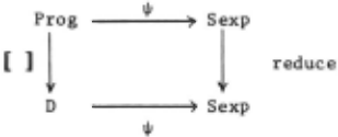
Thus we have seen that the function reduce simu lates the semantic function [ ]. If ~ were a one to-one function 11 then we could compute [ ] by the equation [p]z(~ ·reduce·~)[p]. But~ is not one to-one since ~[J ]·J for any a Type. However, we note that ~xtype?Prog+SexpxType such that (~xtype) [p]s(~[p], type[p]) is one-to-one. Hence we can
compute [ J by the scheme [p]=(~xtype)- 1 [reduce [~[p]], type[p]]. (Note that [ ] preserves type.)
4.3 Concluding Remarks
We believe that we have successfully set a theor etical foundation for program synthesis. It is not difficult to implement our procedure, and we wish to encourage the interested readers to actu ally implement it. In fact, at a suggestion of the author, [Goto 1978] has implemented a system of program synthesis. However, his system differs at an essential point from the one described above, and, at present, no proof exists which guarantees the correctness of the program synthesized by Goto's system. The possibility of using �~del interpretation as a tool for program synthesis has also been suggested by [Kreisel 1977]. [Takasu 1978] also studies the application of �~del inter pretation to program synthesis using the formalism of Gentzen's sequential calculus.
Since the basic data type of Prog is natural num ber, it may appear that such data types as list, stack etc. cannot be dealt with in our formalism. However it is not the case, and we can treat these data types as well by treating them as abstract data types. We wish to discuss this point further in a paper to be published later.
ACKNOWLEDGMENTS.
The author wishes to thank Professor Satoru Takasu of Kyoto University for many stimulating dis cussions with the author. The author wishes to thank Mr. Hayao Nakahara for correcting errors in the original definition of the function reduce.
@inproceedings{ijcai1979p166,
  title     = {Towards a Mathematical Theory of Program Synthesis},
  author    = {Sato, Masahiko},
  booktitle = {Proceedings of the Sixth International Joint Conference on
               Artificial Intelligence, {IJCAI-79}},
  publisher = {International Joint Conferences on Artificial Intelligence},
  editor    = {Bruce G. Buchanan},
  year      = {1979},
  month     = {8},
  url       = {https://ijcai.org/proceedings/1979/166},
}
TY - CPAPER TI - Towards a Mathematical Theory of Program Synthesis AU - Sato, Masahiko T2 - Proceedings of the Sixth International Joint Conference on Artificial Intelligence, IJCAI-79 PB - International Joint Conferences on Artificial Intelligence PY - 1979 UR - https://ijcai.org/proceedings/1979/166 ER -Copied
Machine-readable versions of this paper, for tools and AI agents:





