
RE-EXAMINING PHYSICAL CONSTRAINTS
Proceedings of the Fifth International Joint Conference on Artificial Intelligence. Vision.
© 1977 International Joint Conferences on Artificial Intelligence
Abstract
- Horn, Berthold K. P. (1970), "Shape From Shading: A Method for Obtaining the Shape of a Smooth Opaque Object from One View", MAC TR-79, M.I.T. Project MAC, November 1970. (See also: Horn, Berthold K. P., "Obtaining Shape from Shading Information", In Tile Ps'JCAoloK'J of Computer Vision, P . H . Winston (editor), McGraw-Hill, 1975, pp 115-155.)
- Horn, Berthold K. P. (1975), "Image Intensity Understanding". AI-MEMO 335, AI Laboratory, MIT, August 1975. (See also:. Horn, Berthold K. P., "l)nderstandlng Image Intensities", In Artificial Intelligence, Vol 8, 1977 <in publication>)
- Huffman, David A. (1971), "Impossible Objects as Nonsense Sentences", In Maclttne Intelligence 6, R. Meltzer and D. Michie (editors), Edinburgh University Press, pp 295-323.
- Huffman, David A. (1975), "Curvature and Creases: A Primer on Paper", Proceedings of Conference on Computer Graphics, Pattern Recognition and Data Structures, May 1975, pp 360-370.
- Mack worth, Alan K. (1973), "Interpreting Pictures of Polyhedral Scenes", In Artificial Intelligence, Vol 4, 1973 pp 121-137. IJCAI
- Marr, David Be Pogglo, Tomaso (1976), "Cooperative Computation of Stereo Disparity", AI-MEMO 36i, AI Laboratory, MIT, June 1976.
- Woodham, Robert J. (1977), "Reflectance Map Techniques for Analyzing Surface Defects In Metal Castings", Ph.D. Thesis, AI Laboratory, M.I.T., <In preparation> Vision-S: 1-/oorlham
References were extracted automatically from the PDF and may contain errors.
Full text extracted automatically from the PDF; figures, tables and equations may differ. The PDF is the version of record.
RE-EXAMINING PHYSICAL CONSTRAINTS
One can formulate the probltm of determining the point in gradient space (p.q) corresponding to the Image Intensity point I(x,y) analytically as has been done In <Horn 1970,1975>. This work will not be reviewed here. Instead, the formal nature of the computation will be put aside In order to first re-examine its basis In the physical world.
Two constraints of Importance can be Identified:
- A given point on a physical surface has a unique orientation In space.
- Matter Is cohesive. It is separated Into objects. The surfaces of objects are generally smooth compared with their distance from the viewer.
The reader wl11 note that these are essentially the same two constraints <Marr and Pogglo 1976> use as a basis for their computation of stereo disparity. As In their paper, the goal is to translate the above two physical constraints Into rules for how points in an Image can be matched to points In gradient space.
In their most general form, these rules can be expressed as:
- UNIQUENESS: Each image point may be assigned to at most one location in gradient space
- CONTINUITY: Surfaces vary smoothly almost everywhere. Only a small fraction of the area of an Image Is composed of boundaries that correspond to discontinuities of surface.
The task ahead Is to demonstrate that these rules can be explicitly embedded In a computation. The result is an algorithm which attempts to achieve a global correspondence between Image points and points In gradient space via local, Interactive constraints.
It has become fashionable to call such algorithms "cooperative" after similar phemomena in physics. Perhaps the reader will be more comfortable If the algorithm Is presented as a "relaxation scheme". Nonetheless, what Is Important Is to get the flavor of how local constraints can propagate back and forth to globally constrain possible matches between Image points and points In gradient space.
SPECIFYING LOCAL CONSTRAINT
The basic equation
Is one equation In the two unknowns p and q. With this equation alo.ne, the gradient corresponding to a particular image point is constrained to lie on a one parameter (family of) contour(s) in gradient space. The goal is to apply further constraint In order to assign a unique location In gradient space to each Image point.
The essential physical constraint to be exploited is the assumption that, compared to the viewing distance, surfaces vary smoothly almost everywhere. This surface smoothness assumption Is translated Into monotonlclty rules on changes to view angle and changes to direction of steepest descent permitted between (closely spaced) Image points.
One can 111ustrate how physical constraint adds additional constraint to the possible gradient space solutions to the basic equation I(x,y) · R(p,q). Suppose, two (closely spaced) Image points (x 1 ,y 1 ) and (x 2 ,rz) are hypothesized to correspond to object points on the same section of smooth surface. Further, suppose that the view angle Increases In going from (x 1,y1) to (x 2 ,y 2 ) and that the direction of steepest descent decreases In going from (x 1 ,y 1) to (x2,y2). Let (p 1.q1) and (pz,qz) be the gradient locations corresponding to (x 1.y1) and (Xz,yz).
Suppose, further, that the basic equation l(x,y) · R(p,q) constrains (p 1 ,q 1 ) and (p2,q2) to lie on the contours C1 and Cz respectively as shown In figure 3.
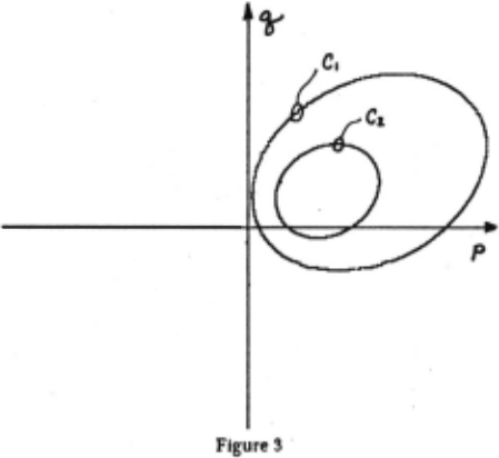
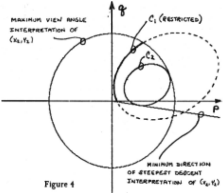
Figure 4 shows, superimposed on the two contours of figure 3, the gradient space circle corresponding to the maximum view angle Interpretation of (p2,q2) and the gradient space line . corresponding to the minimum direction of steepest descent ' Interpretation of (p2,q2). Since the view angle Increases in going from (x 1,y1) to (x2,y2), the contour of permlssable (p 1 ,q 1 ) can be restricted to Include only those gradient points on C 1 lying on or within the circle of the maximum view angle Interpretation of (p2,q2). Similarly, since direction of steepest descent decreases In going from (x 1,y1) to (x2,y2), the contour of permlssable (p 1,q 1) can be restricted to Include only those gradient points on or above the line of the minimum direction of steepest descent Interpretation of (p2.q2). Thus, without any additional constraint on (p2,q2), the assumed monotonlclty relations between (x 1,y1) and (x 2 ,y 2 ) have been applied to the topography of the reflectance map to constrain the possible. Interpretation of (p 1,q 1) to include only those points of C 1 Indicated by the solid line of figure i.
Let (r .f) denote the polar representation of the gradient space point (p,q). That Is: r~
Generalizing from the above illustration, th~ following two rules are stated:
RULE I: CHANGES IN VIEW ANGLE
Let I 1 ,1 2, .·. ,1" be a set of (closely spaced) image points hypothesized to correspond to object points on the same section of smooth surface that are monotonically non-decreasing in view angle. Let C 1 ,C2, ... ,Cn be the corresponding set of gradient contours determined from the reflectance map. Then, each contour C; can be further constrained such that, for each (r,B) t C;. I · 2,3, ... ,n-l
Similarly, If 11,12, ... ,1. Is hypothesized to correspond to a set of object points on the same section of smooth surface that are monotonically non-increasing In view angle, then each contour C; can be further constrained such that, for each (r,l) · C;, I · 2,3, ... ,n-l
RULE II: CHANGES IN DIRECTION OF STEEPEST DESCENT
Let I 1,1 2, ... ,1" be a set of (closely spaced) image points hypothesized to correspond to object points on the same section of smooth surface that are monotonically non-decreasing in direction of steepest descent. As above, let C1,C2, ... ,Cn be the corresponding set of gradient contours. Then, each contour C; can be further constrained such that, for each (r,l) e C;. I · 2,3, ... ,n-t
Similarly, If 11,12, ... ,In Is hypothesized to correspond to a set of object points on the same section of smooth surface that are monotonically non-increasing In direction of steepest descent, then each contour C; can be further constrained such that, for each (r,B) · C;. I · 2,3, ... ,n-l
HYPOTHESIZING MONOTONICITY RELATIONS
It Is now time to turn to the question of how to hypothesize monotonicity relations between selected image points. To begin with, consider the worst possible approach. For some small value of n, one might explore all possible orderings, with respect to both view angle and direction of steepest descent, of selected (closely spaced) Image points 1 1 ,12, ... ,1 .. The hope would be that only a small fraction of those orderings would have admissable Interpretations (ie. Interpretations that included at least one gradient point for each Image point). The constraints Imposed by each local Interpretation would propagate to neighboring sets of selected Image points to provide further mutual constraint. Again, the hope would be that propagation of local constraint would converge to a correct global Interpretation while "incorrect" propagations would (quickly) die out.
Consider a second possible approach. Suppose a particular surface interpretation is forced onto the data. Such an Interpretation would provide a framework to (partla·lly) order selected (closely spaced) Image points with respect to changes in both view angle and direction of steepest descent. Instead of allowing all possible orderings to compete, this second approach pursues a particular Interpretation. Again, the hope would be that propagation of local constraint would converge to a single global Interpretation that represents a simple distortion of the particular Interpretation being forced. (Here, simple distortion Implies any surface that preserves the assumed monotonicity relations concerning changes to view angle and changes to direction of steepest descent.)
The method actually Implemented corresponds to this second approach. The program has a small set of Interpretations It Is willing to pursue. Some are quite rigid, others are quite flexible. In the next section, a specific example is presented. For now, a brief analysis is given to show of how convexity can be used to hypothesize monotonlclty relations between (closely spaced) image points.
By partially differentiating the basic equation I(x,y) · R(p,q) with respect to X and Y we obtain two equations which can be written as the single matrix equation:.
Gj- ~: ::Jt::J . (subscripts denote partial differentiation). Similarly, the two first-order equations dp · p1dx + PvdY and dq · q.dx · qvdY can be written as the single matrix equation:
Recalling the original definitions of p · artax and q · iJf/iJy, observe that Pv · q. (for smooth surfaces, the order of differentiation can be interchanged). Thus, one can define a matrix H by:
H Is the standard Hessian matrix (which captures the notion of surface curvature). The first observation to be made is that smoothness guarantees that H Is symmetric. Thus, it Is reasonable to ask under what conditions Is H positive semidefinite (A real symmetric n x n matrix A Is positive semidefinite if and only If x 1 Ax ~ 0. for all vectors x in R".) Now, H Is positive semidefinite If and only if z · f(x,y) is convex. This result Is used to show how convexity adds constraint. Suppose z · f(x,y) Is convex. Thus, H Is positive · semidefinite. Multiplying the two matrix equations on the left by (non-zero) [RP Rql and (non-zero) [dx dy] respectively, gives the two inequalities:
This first inequality can be viewed as an additional a priori constraint on the contour In gradient space of possible solutions to the basic equation I(x,y) · R(p,q). The tangent vector [Rp,Rql to the contour of constant reflectance at any point (p.q) hypothesized to be a solution to the basic equation I(x,y) · R(p,q) must have a non-negative component in the direction of the tangent vector [I,,Iyl to the contour of constant Intensity at (x,y).
The second Inequality can be viewed as an additional constraint on the possible movement [dp,dq] in gradient space corresponding to a movement [dx,dy] In the Image. As above, the vector [dp,dq] must have a non-negative component in the direction [dx,dy]. Thus, by choosing [dx,dy] appropriately, it is possible to guarantee either the sign of the change to the view angle or the sign of the change to the direction of steepest descent.
ACHIEVING GLOBAL CONSTRAINT
Regardless of what mechanism is used to hypothesize (local) monotonicity relations between points in image space, it is still necessary to embed that mechanism in a computation to achieve global constraint. The Implementation approach taken here is admittedly ad hoc. The program selects nine points in a simple 3 x 3 square pattern as Its basic set of (closely spaced) image points. This pattern serves as the set I1h, ... ,In for applying the local con.stralnt criteria (Rules I and II). First, however, the set 11 ,12, .·. ,1" is passed to the chosen hypothesizing routines to be · (partially) ordered with respect to view angle and direction of steepest descent. The reflectance map R(p,q) Is then used to determine the Initial contour of possible gradient space locations for each point 1;. Rules I and II are interatively applied to these contours until no further mutual constraint is provided.
The above describes the bask application of local constraint to each 3 x 3 template. The selection of successive 3 x 3 square patterns Is allowed to overlap. Thus, each image point I; will eventually belong to nine templates. Each time a particular image point I; is further constrained by the application of local constraint to a template of which it is a member, each of its eight other templates is marked for reconsideration. Before moving on to a previously unconsidered template local constraint is applied recursively to each marked template, with additional marking added as required, until no marked templates remain to be reconsidered. Each time an Image point I; is considered, any additional constraint on the gradient space contour of possible solutions to the basic equation I(x,y) · R(p,q) propagates through this local filtering mechanism to all other image points under consideration.
The next issue to arise is the question of how to terminate the growth of templates. Currently, the program terminates only when some image point under consideration has no admissable gradient space interpretation, in which case the "forced" interpretation Is deemed to have failed, or when all boundary points to existing templates have view angle greater than some preassigned value, in which case the surface is deemed to be too oblique for further expansion. Clearly, these termination conditions are not adequate for a general surface analysis routine. The question of termination also raises deeper issues. How important are boundaries to surface interpretation? How can a complex surface be segmented into simpler (convex/concave) subsections? How does one handle the inherent indentation/protrusion ambiguity In trying to piece together surfaces? These Issues must be dealt with. But, for now, let us consider a specific example in order to illustrate the method in operation.
AN EXAMPLE
Consider the simple example of a "Lambertlan· sphere lllumlnated by a single distant light source. The intensity space to gradient space correspondence will be derived analytically and then it wlll be used as a basis for judging the performance of the computation.
The first task Is to generate a reflectance map. To do this, a reflectivity function must be specified. Now, the term Lambertian refers to a phenomenological model of a perfect diffuse reflector such that the surface appears equally bright from all viewing directions. For such a surface, the reflectivity depends only on the forshortenlng effect of the varying angle of incidence. In particular, the reflectance function .(i,e,g) is given by:
This reflectivity function is transformed into a reflectance map by simply recalling the expression derived earlier for cos(i). The reflectance map Is thus given by:
The second task is to determine the local surface orientation of each image point. In the example, this result Is particularly easy to obtain. Let the object sphere be centered at the origin and have radius r. Thus, the equation of the sphere Is: x2 + y2 + 12 · r2
Elementary calculus will verify that the vector (x,y,z) defines an (outward) normal at each point (x,y,z) on the surface. The appropriate gradient is obtained by rewriting this normal as (-x/z,-y/z,-1). Now, for each (x,y), there are actually two possible z values to be considered. Note, however, that in this example the hemi-sphere actually in view corresponds to negative values of z (recall figure 2).
The parameters of the image forming system can be factored out by assuming that the image intensity has been normalized to correspond directly to reflectivity. In this case, the intensity recorded at each image point (x,y) is equal to the value of the reflectance map at the corresponding (p,q). Thus, the equation for image intensity is:
Finally, the mechanism by which monotonicity relations were hypothesized for this example must be specified. One additional assumption was used. The algorithm assumes that it knows at least one Image point corresponding to an object point oriented directly facing the viewer. Now, let such a point define a pseudo-orlgtn in image space. Since the view angle is assumed to be zero at the pseudo-origin, the only possible interpretation Is that, In a particular direction, the view angle Is locally non-decreasing with Increasing Image distance from the pseudo-origin. In general, one can not hope to assert any local monotoniclty relation on direction of steepest descent based on angular position about the pseudo-origin. If, however, the surface is known to be convex, the direction of steepest descent Is (locally) non-decreasing with increasing angular position about the pseudo-origin. For the example, the set of image points 11,12, ··· ,1" was ordered In view angle according to their distance In Image space from the pseudo-origin and ordered In direction of steepest descent according to their angular position about the pseudo-origin. Applied together, these hypothesis rules are equivalent to the strong assumption that the surface in question Is a convex solid of revolution.
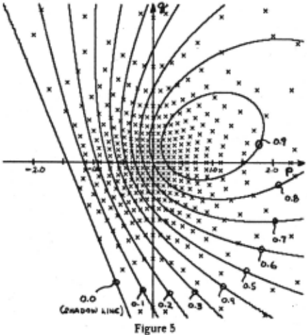
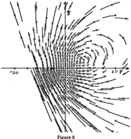
For the example, Ps · 0.7, qs · 0.3 and R · 60. A 128 x 128 test Image was considered. The algorithm was applied to this image using 3 x 3 square templates sampled at an image spacing of 5 points (in both X and Y). The pseudo-origin was defined as x · 0 and y · 0. The results are first presented as a pair of figures . Figure 5 shows the reflectance map R(p,q) · cos(i) drawn as a series of contours (spaced 0.1 units apart). Superimposed are crosses marking the known gradient points (p,q) corresponding to the Image points (x,y) sampled from the Image. All gradient points to the left of the contour R(p,q) · 0.0 correspond to surface points oriented more than 90° away from the direction of Incident illumination and hence to the self -shadowed region of the sphere. Figure 6 shows the restricted subsection of contour determined for each sampled image point. Again, crosses are superimposed to illustrate how well the algorithm has performed. The crosses mark the correct gradient points, determined analytically, while the corresponding subsection of contour marks how well the algorithm has Isolated those points.
DISCUSSION
The ultimate criteria for judging the performance of this method Is, of course, to discover whether It can be used to solve Interesting problems. For now, however, the discussion Is restricted to some simple statistics and some qualitative observations.
How well . has the algorithm performed on this example? To answer this question, the freedom remaining at each image point I; can be examined. Since each point in gradient space defines an orientation, this freedom can be characterized by the angular spread remaining In the corresponding gradient contour C;. This freedom has been measured in two ways. First, define the angular spread In local surface orientation at Image point I; by:
Second, define the angular spread In view angle e at image point 1;:
(View angle Is useful because It determines the degree of surface forshortening at each Image point. Knowing the view angle, one can calculate the area of surface equivalent to a given area of Image.) To tabulate the results, the sample points were split Into two classes. First, consider all sample points within 45° view angle (le. lying within gradient space circle p 2 · q 2 · I). Second, consider all sample points within 60° view angle (le. lying within gradient space circle p 2 · q 2 · 3). Table I summarizes the results:
| Points Within 45° View Angle | Points Within 60° View Angle | |
|---|---|---|
| Local Surface Orientation: | ||
| Mean Angular Spread | 8.9° | 9.9° |
| Standard Deviation | 6.10 | 7.0° |
| Best Case | 0.5° | 0.5° |
| Worst Case | 36.3° | 41 .~ |
| View Angle: | ||
| Mean Angular Spread | 4.~ | 5.0° |
| Standard Deviation | 2.4° | 2.5o |
| Best Case | 0.5° | 0.5° |
| Worst Case | 10.9° Table I | 11.9° |
Note that these measures refer to total angular freedom. If a choice algorithm Is adopted which selects the "correct" answer to be at the midpoint of the angular spread, this choice is guaranteed to be no more than half the angular spread in error. Thus, the .upper right portion of table I can be interpreted as follows:
On tlte ·average, try sampling at an image spactng of 5 points in X and Y, tlte algoritltm was able to position image points, co.rrespon~ing to surface potnts less titan 60° in view angle, to wttltin 5 of tiJttr trut orientation tn space. Tltt standard dtviattoTJ of tAts mtasurt ovtr all suclt points was J.5° while tAt worst cast point was located to wttiJin 2f of tts true orientation tn space.
The performance of the algorithm depends critically on two factors: the ability to hypothesize monotonlclty relations between selected image points and the topography of the reflectance map. The discussion of convexity gives some Indication of how one can use a priori assumptions about surface geometry to specify monotonltlty relations. In any event, given a particular hypothesis mechanism, the algorithm generates a constrained Interpretation consistent with that hypothesis mechanism (or demonstrates that no such consistent interpretation is possible).
The topography of the reflectance map Is determined by two factors: the local photometry of the surface being viewed and the light source, object surface and viewer geometry. In general, one would not expect to have much control over the local photometry of the surfaces being viewed. In principle, however, the user is free to vary the light source and viewer geometry to achieve optimal results with the algorithm. This approach has proven particularly useful In extending these techniques to the problem of Inspecting for surface defects in metal castings (where It Is feasible to construct Inspection stations with Independently controllable light sources <Woodham 1977>).
CONCLUSION
The notions of local surface orientation, gradient space and reflectance maps represent Important conceptual tools for Image analysis. The beauty of the gradient space formulation is that it allows one to formulate physical constraints on the object surface as simple geometric constraints on the gradient space contour of possible solutions to the basic Image forming equation I(x,y) · R(p,q). The beauty of the "cooperative" algorithm Is that It provides a simple mechanism for propagating these geometric constraints.
ACKNOWLEDGEMENTS
I wish to thank Berthold K. P. Horn, Mark Lavin, Tomas Lozano-Perez, David Marr and Patrick Winston for help with the ideas presented In this paper. Anna R. Bruss provided valuable proof-reading assistance. This research was conducted at the Artificial Intelligence Laboratory of the Massachusetts Institute of Technology. Support for the laboratory's artificial Intelligence research Is provided in part by the Advanced Research Projects Agency of the Department of Defence under Office of Naval Research contract number NOOOI4-7!i-C-0643.
@inproceedings{ijcai1977p149,
  title     = {RE-EXAMINING PHYSICAL CONSTRAINTS},
  author    = {},
  booktitle = {Proceedings of the Fifth International Joint Conference on
               Artificial Intelligence, {IJCAI-77}},
  publisher = {International Joint Conferences on Artificial Intelligence},
  editor    = {Raj Reddy},
  year      = {1977},
  note      = {Vision},
  url       = {https://ijcai.org/proceedings/1977/149},
}
TY - CPAPER TI - RE-EXAMINING PHYSICAL CONSTRAINTS T2 - Proceedings of the Fifth International Joint Conference on Artificial Intelligence, IJCAI-77 PB - International Joint Conferences on Artificial Intelligence PY - 1977 UR - https://ijcai.org/proceedings/1977/149 ER -Copied
Machine-readable versions of this paper, for tools and AI agents:
 Welcome
 Future Conferences
 AI Journal Division
 IJCAI Proceedings
 About IJCAI
 IJCAI Awards