Set Variables

1. Introduction

For many theorems the main difficulty in the proof is in defining~ particular set. Once that is done the proof often proceeds rather easily. For example, in

If we let A= (x: x < 0}, then we are left with the trivial subgoal:

Or, if we are proving the intermediate value theorem,

Theorem. If f a < x < b, f (a) < 0, f(i) = Q for some X Figure 1) is continuous for and f(b) > 0, then between a- and b. (See

Using the least upper bound axiom,

LUB Axiom. Each non-empty bounded set A of real . numbers has a least upper bound.

And if we let

then again the proof is rather straightforward (but harder than the last example). The question of course, is how to select A?

* This work· was supported by National Science Foundation Grant MCS 76-23760.

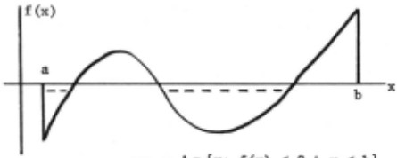
Figure 1 The Intermediate Value Theorem

There are several other theorems in analysis, such as the Reine-Borel Theorem where the chief diffi­ culty lies in defining a particular set. Also a similar situation comes up again and again in other parts of mathematics, and in application areas such as program verification and program synthesis.

The problem of finding a value for a set var­ iable A, is of course equivalent to the problem of giving a value to a one place predicate vari­ able P .

This is a part of higher order logic, and as such can be attacked by the systems and ideas of Huet [3], Pietrzykowski [10], Haynes and Henschen [7], Andrews [11], etc. But these are very slow for many simple proofs. For example, Huet's beautiful system [3] is forced into double split­ ting on the rather easy theorem given in Example 4 below. (Even a human has trouble applying his procedure to this example.)

In this paper we describe a procedure which attempts to overcome this difficulty. It is less general than those referred to above; it usually applies only to a part of second order logic (but an important part); and it seems to be must faster when it applies . Ours is more in the spirit of J. L. Darlington's "F-Matching", but different in method and scope.

Our methods are not domain specific, not just a collection of heuristics for finding sets in a particular area like analysis. They can be used to prove theorems (such as the intermediate value theorem) in analysis where the set A is a set of real numbers, as well as theorems in topology where the set A is a family of sets, and theorems from program correctness, or from other areas where set variables are to be instantiated.

In Section 2 we give some preliminary examples and in Section 3 we describe our rules for gener­ ating the desired set A. They consist of basic rules which apply to simple formulas and co~ng rules for combining the results from the basic rules .

One of our goals in this work is to avoid in­ descriminant matches (or attempts at matches) be­ tween formulas such as (t € A) and P, (where P is first order), but rather to allow such a match only when (t € A) and P are somehow "connected". In this way the search is drastically reduced. Our basic rules (see Figure 2) are a partial attainment of this goal.

Our methods are "maximal" in that they usually generate the largest set with the desired proper­ ties (if there is one). Of course some theorems

such as,

~A[ (A is dense in R) 1\ ( (R-A) is dense in R))

has no maximal (nor minimal) solution for A. Al­ so in some cases there is more than one maximal solution (see Example 5, Section 3), even infin­ itely many solutions . However, we believe there is a wide class of interesting cases that have a unique maximal solution, or at most one or two

maximal solutions.

Our procedure utilizes the automatic prover described in [1) as a "control" (see Section 4) for generating the desired sets. But one can follow this presentation without full knowledge of that paper .

In actual practice the prover makes two passes on a theorem: first to define the set A; second to prove the resulting theorem, after the set A has been instantiated. Thus the procedure is sound i.e. there is no danger of it producing a false solution since the solution is always verified .

In Section 5 we give excerpts from somemajor examples which are described in more detail in [ 0). In Section 6 we make several comments .

These methods do not satisfactorily handle the induction axiom. This is discussed in Section 6 of [0). Some completeness proofs for these methods are given in Appendix II of [0).

2. Some Preliminary Examples

We are concerned here only with cases of the form

where the variable A is to be found (i.e., given a value). Since ((VAP(A)) ~C) is equivalent to 3 A(P (A) ~ C), we will usually act as if our theorem is already in the form .3 A P (A) . Theorems where A is a constant can usually be handled as first order logic.

We will treat only the case where there is but one such set variable A. However our methods will-often work for theorems with many such

variables.

Once the set A has been found, the theorem becomes first order, and hopefully not too diffi­ cult. That will often be the case. However, it is well known that automatic theorem proving for first order logic is a most challenging and un­ resolved task.

It is our objective here to automatically de­

fine such variables.

Let us look at some examples before giving the rules. These fragments help illuminate the procedure. More substantial theorems will be given later in Section 5.

* Provided that A does not occur in c.

Example 1. 3 AVx(xEA~x~O).

Solution: A= (x: x ~ 0).

This is the simple theorem which states that "there is a set A for which, for each x in A, x is non-positive". Clearly, one such A is the set of all non-positive reals, and that is exactly what is returned by our program. When this value is substituted for A the theorem reduces to the trivial subgoal (x < 0 ~ x < 0), which our pro­ gram quickly verifies as true.

Solution: G= (A: 3B (B € F 1\ A~ B).

This example is very much like the previous one, except that G plays the role of A, A plays the role of x, and 3 B (B € F 1\ A c B) plays the role of X < o. Notice that the variable G iS a II family" Variable rather than a 11 Set 11 Varia­ ble. Thus we have (technically) proved a theorem in third order logic, although it is for all prac­ tical purposes a theorem in second order. It is desirable, we believe, to keep formulas like 3 B (B € F 1\ A c B) together during the process­

ing and this is-what our program usually does.

Next we consider a theorem of a little more

substance .

Example 3.

It is now time to note · that A= 0 is a per­ fectly good solution to Example 1. However, A= 0 will !!£!_ work for Example 3; here we must include in A at least the point a. We prefer to put all we can in A, thus getting a maximal

solution.

In Example 3 there are two types of occurr­ ences of A: the "EVEN'' occurrence y € A, and the "ODD" occurrence in (x e A- P(x)1 2 · The ODD occurrences are used to determine A (according to the rules in Section 3), and the EVEN occurr3 ences are just checked after A has been defined . Accordingly when the solution given is put in for A we get

2 Note that (x€A~P(x)) is equivalent to (x t A VP (x)). If A does not occur in B (ex­ cept possibly as a skolem argument -- see foot­ note 4) then A is in an EVEN position of A/\ B, AVB, (B ~A), B, and A itself; and A is in an ODD position of (A~B), (-A), and B. Also an EVEN position of an EVEN position is EVEN, ODD of ODD is EVEN, ODD of EVEN is ODD, and EVEN of

ODD is ODD .

3 This is equivalent to putting the universal set U for A for the EVEN occurrence and inter­ secting it with the set (x: p(x)) gotten for

the ODD occurrence.

in which the ODD part is now trivial and the EVEN part is yet to be checked (but can be).

The next example will illuminate that point.

Example 4 .

ODD EVEN ODD

Solution: {x: x#aAx#c}.

The two ODD occurrences give respectively (x: x# a} and {x: x# c}, and the EVEN occurr­ ence gives U (using the rules of Section 3) which are combined (by the "combining rules" of Section 3) into the given solution.

Notice that this is not the only solution. There are many others such as {x : a < x < b}, {x: a < x < b}, {b}, but none of these are maxi­ mal. Our ;ethod gives the maximal solution if there is one.

We could have developed a minimal theory, getting the smallest sets, by using the EVEN occurrences of A instead of the ODD, but we have a slight preference for maximal . Intermed­ iate sets would be difficult to produce automatic­ ally. Only when we work against the extremes do we reduce the complexity of the problem.

3 . Set Building Rules

3.1. Basic Rules

Our rules for generating maximal sets are of two kinds: (i) basic rules and (ii) combining rules. The basic rules give solutions to certain sub formulas of the form: (x € A), (x f. A), (x € A * p (x)), and the combining rules consoli­ date these basic solutions into one general solution, depending on the placement of these sub­ formulas in the theorem. For instance, in Example 4 above, the subformulas (a i A), (b € A), and (c f. A) were connected by " A", so the corres­ ponding solutions {x : x#a}, U, and (x: x#c} were intersected to obtain the general solution {x: x#aAx#c}.

Figure 2 gives our first set of basic rules. More are added later. In Figure 2 the subformulas

shown are expected to be in an EVE~ position of the theorem being proved, and the theorem itself 4

is to be in skolemized form .

Also it should be noted that these rules can­ not handle an expression in A until it is reduced to the form (x € A) . (This includes the cases x f. A and (x € A* C).) This reduction may re­ quire the use of hypotheses, definitions, and lemmas .

4 see App. 1 of [1) for a complete description of skolemiza.tion, or footnote 12 of [2).

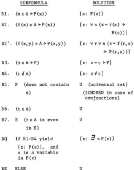
	SUBFORMULA	SOLUTION
B 1.	(x € A* P (x))	{z: P(z)}
B2 .	(f(x)eA*P(x))	( z : Y s (z = f (s) * P(s))}
B2'.	(f(x,y) eA*P(x,y))	{z: YrYs (z=f(r,s) * P (r, s))}
		{z : z=t *P}
B4.	(t t A)	{z: z#t}
BS.	P (does not contain A)	U (universal set) (IGNORED in case of conjunctions)
B6 .	(teA)	u
B 7 •	E ( t € A is even in E)	u
BQ	If Bl-B4 yield { z: P(z)}, and s is a variable in P (z)	{z: :J sP(z)}

Figure 2

BASIC RULES

The rules of Figure 2 operate under the restrictions listed in Table I below:

1. The Rules Bl-BE apply to subformulas in EVEN positions of the theorem. A is a set vari­ able to be instantiated. It is the only set variable (indeed the only higher order vari­ able) in the theorem. A occurs only in the form (t € A), or as a skolem function argu­ ment.
2. In Bl x is a skolem function 4 of A, A does not occur otherwise in P (x), x does not occur elsewhere in the theorem, and no other varia­ ble occurs in x (i.e., xis a skolem function of no other variable but A).
3. In B2, B2', x and y are skolem functions of A, A does not occur otherwise in P(x) or P(x,y), x and y do not occur elsewhere in the theorem, and no other variable occurs in x, y, f(x), or f(x,y).
4. In B3, A does not occur in t or P.
5. 4 . In B4, A does not occur in t
6. In BS, A does not occur in P.
7. In B6, A does not occur in t.

BE

ELSE

u

1. In B7, every occurrence of an expression of the form (t € A) in E, is in an EVEN position of E, A does not occur in t. A cannot occur in E except in one of these subformulas (t € A).
2. In BQ, s is a variable in P(z), but does not occur elsewhere in the theorem.
3. In BE, the subformulas have the form of Bl-B7 or BQ, but the restrictions 1-8 are not sat­ isfied.

Table I

In Rules Bl and B2, "x" is required to be a skolem 4 function of A, and not appear in the rest of the theorem. That is to say the sub­ formula V x (x € A + p (x)) occurs in an EVEN position of the theorem within the scope of A. See Section 7 of [0] for a further discussion of this and some means of easing these restrictions on x. Similarly for x and y in B2'.

Note that when the term "t" is not quanti­ fied within the scope of the quantification of A, as in :SA (t € A+ P(t)) then by Rule B3, we do not derive the solution (z: P(z)} as was done in Rule Bl, because it is not the maximal solution. Rather the maximal solution is (z: z= t + P(t)} as given by Rule B3. Rule B4 acts similarly.

Rules B5-B7 give the universal set U as a solution for expressions of the form (t € A) and for EVEN combinations of these. Since (U n A 0 ) = A 0 , the effect is to ignore expressions that give the solution U whenever they are con­ joined (connected by " 1\ ") to other expressions.

These rules and those in Sections 3. 2-3.6 are supported to some degree by the proofs in Appendix II of [0] . Our objective is to find maximal sets for a few basic forms, and to give combining rules that retain that maximality.

3.2. Combining Rules for Conjunctions

We will first give in Figure 3, three com­ bining rules for conjunctions before giving others. These three rules with the basic rules of Figure 2 have been sufficient to prove a num­ ber of interesting theorems. Even our extended list of combining rules is by no means complete; we are now in the process of trying to validate and extend both the basic and combining rules.

• (i) If A 1 is the (only) 5 maximal solution for P(A),
• (ii) and A 2 is the (only) maximal solution for Q(A),

5 If P(A) or Q(A) has solution (see Example 5 this rule still applies solutions A 1 of P(A) Az of Q(A). more than one maximal and Figure 5 below), to at least one of the and one of the solutions

• (iii) and both A 1 and A 2 are obtained from the basic rules of Figure 1, or fro~ combining rules Cl-C3, (or if
• (iii)': P(A) and Q(A) have the intermediate property (see below))
• Cl. then (A 1 n A 2 ) is a maximal solution of (P(A) 1\ Q(A)), if it has a solution,
• C2. and (A 1 n A 2 ) is a maximal solution of (H + P(A) 1\ Q(A)), if it has a solution, provided that "A" does not occur in H,
• C3. and (A 1 nA 2 ) is a maximal solution of ((R V P (A)) 1\ Q (A)) if it has a solution, provided that "A" does not occur in R.

Figure 3

Three Combining Rules for Conjunctions

Definition. We say that a formula subset property (superset property) B and C, if B is a solution of is a subset (superset) of B then solution of P. P has the if for each P and C C is a

Definition. We say that a formula P has the intermediate property if for each B,C, and D, if B and D are solutions of P and B c C c D, then C is a solution of P. -

It is easily seen that if P has the subset property or the superset property then P has the intermediate property, because ~ is a solution of a formula with the subset property (if it has any solution), and U is a solution of a formula with the superset property (if it has any solution).

It is easily shown that the subformula·s in Rules Bl-B5, and BQ, have the subset property, and those of Rules B5-B7 have the superset prop­ erty; and that the conjunction of two formulas with the intermediate property also has the in­ termediate property. Therefore the combining rules of Figure 3 are valid by condition (iii) 1 as well as by (iii), by Theorems 12-13 of Appendix II of [O].

3.3. Combining Rules for Disjunctions

Often there can be more than one maximal ----6solution or even infinitely many For example the theorem

A [V x (x € A + P (x)) VVy (y € A + Q (y))]

has two maximal solutions (z: P(z)} and (z: Q(z)} each with the subset property. (But {z: P(z) V Q(z)} is not a solution~)

When there is m~ than one maximal solution

we will indicate the "maximal solution" as a family ~ of sets. For example, the family of candidate solutions for

6 see Section 3.5 .

Example 5.

P(a) ~ 3 A ([Yx (x € A~P(x)) !\ 3 y (y € A)]

V [Y x (x € A~ Q (x)) !\ 3 y (y € A)]),

is:

Then we must verify that some member of Sf does indeed satisfy the theorem. In this example only {z: P(z)} satisfies.

This brings us to Combining Rules C4-C6 in Figure 4 .

3.4. Further Basic and Combining Rules

Each of the subformulas in the basic rules of Figure 2, except Rule BE, have the intermediate property. This allowed us to use the rathersimple combining rules of Figure 3 for conjunctions . In Figure 6 of [0] we give rules for some cases which do E2! have the intermediate property, and use these to prove some theorems from program verifi­ cation, where internal assertions are not provided by the user but are found by the prove~ (See Example 14 below) _

• C4 . then Sf= {A 1 ,A 2 } is the maximal solution of (P(A) V Q(A)).

Also if

• (iv) P (A) has a maximal solution sr 1 ,
• (v) and Q(A) has a maximal solution sr 2 ,
• (vi) where sr 1 and sr 2 are gotten from C4 - C5, or are gotten from Bl-BQ where the output there is treated as a singleton {AO}'
• C5 . then (sr 1 usr 2 ) is a maximal solution of (P (A) V Q (A),
• C6. 7 and (SJl nn SJ2) includes a maximal solution of (P(A) !\ Q(A)).

Figure 4

Two Combining Rules for Disjunctions

3.5. Infinitely Many Maximal Solutions

We saw in Section 3.3 an example which has two maximal solutions . Others have more, even infinitely many . For example

Example SA.

:3:AYxYy (xEA/\ yEA 7 P(x,y))

If P(x,y) can be "separated", the solution is easy . For example if P(x,y) = p(x) /\ q(y), then the maximal solution is {z : p(z) /\ q(z)}.

However if P (x, y) = (0 < x/2 < y < 2x), then the maximal solutions consist of the infinite family of all the squares of the form

for a > 0. (See Figure 5) Notice that these maximal-solutions may overlap.

Clearly one could not try all of these solutions, in order, as could be done in Example 5. However, as we shall see shortly, our rules can be very effective indeed even when there are infinitely many solutions. -- --- --- --

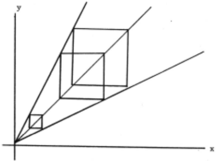
Infinitely many maximal solutions of 3 AYxYy (x€ A !\ YEA 7 P(x,y))

Example SB.

1. 3 AYL 3 yY z [ (Z€ A-7 p(z,y)) !\ q(L,y)]

This is equivalent to (successively):

• 3 A 3 g YLYz[(zEA~p(z,g(L))) !\ q(L,g(L))] 3g 3A[Yz (Z€A-7YLp(z,g(L)))

1. 3 g 3 A [Y z (z € A 7 P (z, g)) !\ Q (g))] .

Now if is a solution for Q(g) then {z: P(z,g 0 )} is a maximal solution (2). At first blush this would seem of little value, since find­ ing such a g 0 is itself a search problem in second order logic, (and since indeed the complete maximal solution of (2) is the possibly infinite family of all such {z: P(z,g 0 )}). However, in many applications the family of maximal solutions is reduced to !_ family of ~ by matches during the proof on other parts of the theorem. This is exactly what happens in the use of the LeastUpper Bound Axiom, LUB, to prove theorems like Example 11 of Section 5.

i· Control

4.1. The Prover as a Control

As mentioned above, the set building rules of Section 3 are used to propose a value for a set variable A and then IMPLY, our automatic prover [1] is used to prove the resulting theorem.

It turns out that the prover is also a con­ venient vehicle for controlling the use of the set building rules. In doing so it proceeds in its normal way to prove the theorem, applying a list of production rules: to manipulate the theorem, to propose subgoals, to manipulate the data base, to match, etc. 8 The set building rules are added

to these production rules.

For example, in proving the theorem,

It first skolemizes and sets up the goal

and then splits it into subgoals (1), (2), (3).

Rule Bl is applied to this subgoal to yield the solution {z: P(z)} for A. This value of A is not substituted for A in the reaminder of the theorem, but rather is placed in the data base, to be combined with other values gotten later.

This subgoal is ignored by Rule B6. (Actually it yields the universal set U, which will bein­ tersected with other sets and therefore" ignored".)

Rule B4 is applied to this subgoal to yield the solution {z: zlb} for A. This too is placed in the data base, and combined with the earlier solution, yielding

8 The reader is referred to [1] for details and examples. For our purposes here the prover des­ cribed in [1] has been augmented by a data base for handling our set variables and interval types (see Section 4. 2). These data base manipulations are in the spirit of those mentioned in [9] and applied in [5,6] and [8].

as the current solution for A.

Since (3) is the last subgoal,the solution (*) is substituted for A in nal theorem, getting the new goal: final the origi-

Now this, which is a first order theorem, is proved as a series of subgoals.

Our intention here is to emphasize the part of the process that builds the set A using the set building rules, and to deemphasize the proof of the resulting first order theorem,

4.2. Interval Types

Before describing other examples in Section 5 we will de~cribe another part of our data base which is called "Interval types" in [ 4] and which plays a crucial part in proofs of theorems in real analysis . This is best illustrated with an ex­ ample .

The skolemized goal is

The prover handles the first subgoal

not by giving some particular value to x, such as 0 or 2 or 1, but rather by storing the entry {x: 0 2} in the data base, indicating that the variable x is now restricted to the inter­ val 0 < x < 2. The prover then goes to the second subgoal

with x still a variable. When this goal is solved, with 1/x, then it must verify that this substitution is consistent with its data base entry, i.e. that 0 ~ 1 ~ 2. ·

Such a data base mechanism is used in the proof of the intermediate value theorem inExample 11 below, and other like proofs in real analysis . This concept which was used in (2], has literally made the undoable doable . Otherwise one is in­ volved in the use of the axioms for the real num­ bers and for inequalities which tend to choke automatic provers not ·using special mechanisms like this.

~· Some Major Examples

Section 5 of [0] summarizes the proofs of several examples. We list here some of those examples and the derivect 9 solution for each.

Example 8. If a set B contains an open neighbor­ hood of each of its points then B is open. 10

Or symbolically

The following lemma is used:

• L: The union of a family of open sets is Open.

The object is to find this family G.

Solution: {Z: Open Z A Z ~ B}.

ll Example 9. If F is a family of open sets covering the regular topological space X, then there exists a family_ G of open sets which covers X and for which G c c F.

The object is to find this family G.

The following definitions are used:

Regular: YAY x (Open A A x e A

OC F: F ~OPEN A Cover F

Cover F: Y x 3 A (A € F A x € A) .

Thus our theorem becomes

(Regular A OC F +- 3 G (OC GA G c c F)) -- ,

9 See Section 6 for a discussion of what was actually proved by the computer on these examples .

10 An open neighborhood of a point x is just an open set containing x. We will use the capital­ ized OPEN to represent the familyJall Open sets. (Union G) is defined to be the set of points

contained in some member of G.

1 lwe will denote by A the "closure" of a set A, and by (; _the_family of closures of members of G, i.e. G= {A: A € G}. Furthermore (H ~ ~ F) means that H is a refinement of F, i.e., each member of H is a subset of a mem­ ber of J, or (YA (A € H +- 3 B (Be FAAcB)). Thus (G ~ ~ F) means Y A (A € G +- -

a B (B 'e F A A~ B)).

in skolemized form.

1. Solution :

The next (rather simple) example is given to show the effect of lemmas on the maximal solution . Let R represent the real numbers and Q the rationals .

Example 10. '3 A (A is dense in R)

This of course has no maximal solution for A. However, if we employ the lemma

then we do get a maximal solution. (See [0]) {z: z ~ Q}=Q.

So a theorem with no maximal solution was given one by the use of the lemma. In other theorems, the maximal solution is often changed (decreased) by the use of lemmas. Indeed that is the case in Example 11 below where a non-maximal (but adequate) solution

is given instead of the actual maximal solution

Example 11. (Intermediate Value Theorem)

If f is continuous for a < x < b, a < b, f(a) ~ 0, and f(b) ~ 0, then f(x)~ 0 for some x between a and b. (See Figure 1) The proof of this requires the least upper bound axiom, LUB:

LUB. Each non-empty bounded set A has a least upper bound.

The object here is to find the set A re­ quired by the least upper bound axiom. The defi­ nition of the set needed here is not at all ob­ vious (even for humans). We believe that the use of a natural deduction prover, such as ours, as a control, is the key to this kind of problem, whereby the prover explores its various subgoals in a natural way and us-es the basic set-building Rules Bl-BQ as they become applicable. Only com­ bining Rules Cl-C3 are applicable in this example so the basic solutions are intersected to obtain the general solution

for A. (See [0] for details.)

The theorem and axiom (in symbols) are:

Instead of the definition of continuity the following two lemmas are used:

• Ll. (Cont fx + V a (a< f(x)

• LZ. (Cont f x + V a (f (x) < a

The "interval typing" described in Section 4.2 played a crucial role in this example. See [0].

This example which was suggested by Peter 12 Andrews is just the theorem

where (a. = 13 ) has been characterized by VD (a. € D + J3 € D), (with the proper typing on D).

Solution: (z: z= (y} + y € A} for F, using Rule B3

The next two examples use some additional Rules from Reference [O]. These are found in Figures 6 and 7 of [O].

In the following example we use Rules Bl and BCl of [O] to obtain the preliminary solution, which is then simplified (by the author) to the solution.

Example 13. 3 A [V x (x € A + x ~ 0)

Preliminary Solution:

Solution:

(z: z > OA 3 N(z=Z·N)}=the set of non-negative-even integers.

12 Private communication .

Example 14. :1[ PVAVK [P(O,x) A (P(A,O)- A= X· y) A (P(A,K) A K '/- 0- P(A+y,K-1))].

This theorem arises from the field of program verification, in a case where the internal assertion P is not given but must be found by the prover. The th;Qrem represents the verification conditions for a simple program which multiplies integers x and y. (See Figure 6)

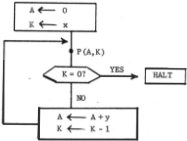
Input assertion: x ~ 0, y ~ 0, integers.

Output assertion: A= x ·y.

Internal aRsertion at ~: P(A,K), to be determined.

Figure 6

Flow Chart for a Simple Multiply Program

In Example 14 we replace the two-place predicate P by a set B of ordered pairs, and skolemize to obtain

Then Rules B6, BZ' and BCZ' are used to obtain,

This solution is then simplified (by the author) to

which corresponds to the predicate P, where

which is the usual interval assertion given by humans for the program dipicted in Figure 6. See [ 0) for more details.

6 . Conunents

Delaying

In our procedure we have employed a concept of delaying, whereby we delay the final determin­ ation of a set A until all parts of the theorem have been processed. Early subgoals place restrictions of the form {z: P(z)} on A, but leave A itself as a variable to be further con­ sidered later. Later subgoals may further re­ strict A, or may force A to take a particular value A (e.g . , by matching) . In this last eventual~ty the program must check that A 0 is

consistent with the earlier restriction {z: P(z)}. This kind of delaying has the marked advantage of not closing off the determination of A by assuming early values for it; but rather keeping it "as general as possible", putting on restrictions only as they are forced. Thus we see that the notions of "maximality" and "delaying" are somewhat analogous.

This concept of delaying is an important one in other parts of automatic theorem proving. Huet's constrained Resolution [3) is an example of it where he delays the higher order unifications until resolution matches have been made. The most general unifier [16) is another example, in that it lets resolution (or whatever prover that uses it) delay as long as possible the assignment of

constant values to variables.

Also our use of· delaying for set variables is entirely analogous to the concept of interval types [2,5,6) explained in Section 4 . 2, when a variable x is restricted to an interval [a< x < b) to satisfy an earlier subgoal, but left a variable to be instantiated or further restricted later . This ·technique has greatly sim­ plified our proofs in analysis, and we expect other such "delaying" methods to be developed.

Relation to the Work of Others

Darlington's program [12,14) has proved Example 8 and other examples using his F-matching. Our procedure has a similarity to F-matching and was partially inspired by talks with Darlington . But it is different especially in its use of the maximality concept which is an outgrowth of the ideas in [ 15, Sec . 10), and in other ways.

This work is of course related to Behmann's decision procedure for monadic first and second order logic [13) 13 . A cursory look at [13] indi­ cates that our solutions are often the same as Behmann's. His methods might be extended to also handle a number of non-monadic cases (as ours do). So it seems that an extensive study of papers on monadic logic is very much in order.

13 J .A. Robinson first pointed this out to me.

The procedures of [3,4,7,10,11) are more gen­ eral than ours, and their research provides a necessary base for this type research; we only feel that our work can be more effective on a limited, but important part, of higher order logic.

Completeness

All of our rules are sound because no matter What value we get for the set variable A, we always verify it with another pass through the prover. The only question, then, is one of completeness.

See Section 7 .5 and Appendix II of [O) for a discussion of, and some proofs on, completeness of these rules .

Implementation

An augumented version of the prover described in [1), which operates in Machine-only Mode (i . e., not man-machine), has been used to prove some ex­ ample theorems. But not all of Examples 1-15 of this paper were actually proved. Examples 1-4, 6-12, were proved outright. Some others could have been proved by minor changes in the program which we are in the process of making; and some require more extensive changes.

Acknowledgment

This work has benefited from conversations with Mike Ballantyne, Mabry Tyson, Peter Bruell, Allan Robinson, Ernie Sibert, Peter Andrews, and Gerard Huet. Also, Peter Bruell has helped de­ velop and implement the computer program.