Computer Proofs of Limit Theorems

COMPUTER PROOFS OF LIMIT THEOREMS

W. W. B.ledsoe, Robert S. Boyer, William H. Henneman

Massachusetts Institute of Technology and the University of Texas

ABSTRACT: Some relatively simple concepts have been developed which, when incorporated into existing automatic theorem proving programs (including those using resolution), enable them to prove efficiently a number of the limit theorems of elementary calculus, including the theorem that differentiable functions are con­ tinuous. These concepts include: (1) A limited theory of types, to designate whether a given variable belongs to a certain interval on the real line, (2) An algebraic simplification routine, (3) A routine for solving linear in­ equalities, applicable to all areas of analysis, and (4) A "limit heuristic", designed especially

for the limit theorems of calculus .

1. Introduction. In this paper we describe some relatively simple changes that have been made to an existing automatic theorem proving program to enable it to prove efficiently a num­ ber of the limit theorems of elementary calculus. These changes include subroutines of a general nature which apply to all areas of analysis, and a special "limit-heuristic" designed for the limit theorems of calculus.

These concepts have been incorporated into an existing LISP program and run on the PDP-10 at the A. !. Laboratory, M.I.T., to obtain com­ puter proofs of many of the limit theorems, including the theorem that the limit of the sum of two real functions is the sum of their limits, and a similar theorem about products. Also computer proofs have been obtained (or are easily obtainable) of the theorems that a continuous function of a continuous function is continuous, and that a function having a derivative at a point is continuous there, as well as limit

results for polynomial functions.

The limit theorems of calculus present a surprisingly difficult challenge for general purpose automatic theorem provers. One reason for this is that calculus is a branch of analysis, and proofs in analysis require manipulation of algebraic expressions, solutions of inequalities, and other operations which depend upon the axioms of an ordered field . It is in applying these field axioms that automatic provers are usually forced into long and difficult searches. On the other hand, a human mathematician is often able to easily perform the necessary operations of analysis without being aware of the explicit use of the field axioms . One purpose of this paper is to describe ways in which automatic provers can also avoid the use of the field axioms and and speed up proofs in analysis. Section 2 ex­ plains how this is done using a limited f~e9ry of types and routines for algebraic simp lflca­ tion and solving linear inequalities.

In Sect1on 3 we present the l1mit-heuristic, give examples of its use, and discuss its "forcing" nature which enables it to curtail combinatorial searches. ·

The reader interested only in resolution based programs should skip Sections 4 and 5 and go directly to Section 6, where we explain how resolution programs can be altered to make use of the limit heuristic and other concepts.

In Section 5 we give a detailed description of a computer proof of the theorem that the limit of the product of two functions is the product of their limits. This proof was made by a pro2ram which is the same as that described in [lj, except that the subroutine, RESOLUTION, in [1] has been replaced by a new subroutine called IMPLY. We have thus eliminated resolution altogether from pur program,replacing it by an "implication method" which we believe is faster and easier to use (though. not complete). This implication method is described briefly in Section 4, and excerpts from actual computer proofs using it are given there and in Section 5.

It appears that some of these ideas may have wider implications than the limited scope in which they were used here. This is discussed in the comments of Section 7 and throughout the paper.

1. Types and Inequalities. In the work des­ cribed in this paper we have used membership ~whereby the type A is assigned to x when­ ever it is known that (x c A).

Let <a b> denote the open interval from a to b, R = <-~ ~ > , P = <0 ~> , and N = <-~-0> . We are primarily interested in Tnterval types, including the types R, P, and N. Thus in trying to prove - -

we would assign the type P (or <0 ~ > ) to x and then try to prove Q(x). -

For example, suppose that we are to prove

One valid approach is to solve for x in

and then try to verify

for that same x. But using matching we would get as a solution of (2) the substitution [b/x], 2 and require (0 < b ~ b < b) in (3), which is impossible. Of course (1) is unprovable with­ out further hypotheses (or axioms) but it can be easily handled by the use of types (which im­ plicitly assumes certain axioms). Our approach in proving (1) is to assign type <0 ~> to b, and then try to prove

1. We use the words "SOME" and "ALL"as our exis­ tential and universal quantifiers. Thus

·'SOME x P(x)" means "for some x P(x)", and

"ALL x P(x)" means "for all x P(x)".

We first solve

by assigning type <0 ~> to x and then solve

(6)

(x<b)

by assigning the type <0 b> to x. The resulting type of x, <0 b>, was derived as the inter­ section of its initial type <0 ~> gotten from (5), and the interval <-~ b>, which would have been the type gotten from (6) alone. Since this intersection is not empty (because b has type <0 ~>), it is assigned as the resulting type of x. Even though the variable x had already been "solved for" in (5) (typed), it remains a vari­ able in the solution of (6) (though limitea-Tn scope) and therefore could be "solved for" again (retyped) . In the examples of Section 5 some of the variables are retyped two or three times, and this greatly simplifies the proofs.

Types are used by the routines SOLVE< and SET-TYPE which are described below.

2.1 SOLVE<

This is a routine for solving linear in­ equalities. (SOLVE< A B) chooses a variable from A or from B and attempts to solve the inequality (A < B) in terms of that variable. If this fails it then chooses another variable and tries again. Since the terms and variables of A and B may be typed, this routine must take into consideration such types and reset the type of the variable when the solution is obtained. In fact the answer is completely given by the new types. The examples below best illustrate this point. If it can show that A is less than B, then the routine wi 11 return the answer "T" whether or not A and B have any variables.

Examples.

INPUT	New Tyle of x Aiven by _soLVE< 8)
A	B
1. X	<-~ 1>
2. X Type x is <0 ~>	<0 1>

In this example the type of 0 in the answer could have been given as <0 (minimum 010 9 )> but we find the intersection form more conve~ient.

Type X iS <0 ~>

Type a is <-~ 0>

Type b is <0 ~>

In the actual theorem proving process, SOLVE< is applied to formulas that have been converted to quantifier free form by the intro­ duction of skolem expressions.3 Precautions are taken by SOLVE< to insure that it does not solve for a variable x in terms of a skolem expression in which x occurs. This is essentially the same precaution taken by J. A. Robinson in his Unification Algorithm [2] .

For example, consider the false statement

The skolem form of this is

The result of a call to (SOLVE< (y x) x) is NIL, since x occurs in the skolem expression (y x).

On the other hand, the theorem

SOME x ALL y SOME z (y < x+z)

which has skolem form

can be proved by a call to (SOLVE< (y x) (x+z)) which correctly assigns type <(Y x)-x ~> to z.

Actually, the routine SOLVE< just retypes a variable in a way that guarantees the solution of the desired inequality.

More extensive routines could easily be written (indeed have been written by others) to solve nonlinear inequalities, but these were not found necessary for proving the examples reported here.

3. A skolem expression is a term whose main function symbol is a skolem function. cf. foot­ note 11 in Section 4 which describes the elimin~ lion of quantifiers by the introduction of skolem functions.

2.2 SOLVE=. This is a routine for solving TTnear equations. Given two arithmetic expres­ sions A and B, it selects a variable x from A or B and trys to solve the equation (A = B) in terms of x. If it succeeds, with answer y, it returns the substitution, [y/x] . Otherwise it selects another variable and trys again, return­ ing NIL if all fail.

2.3 SET-TYPE. This is a subroutine which assigns types to certain skolem expressions. If a formula of the form (A c B) is in a con ­ junctive position of E (i.e., E can be expressed as ((A c B" D) for some D), and if A is a skolem expression which does not occur in B, then (SET-TYPE E) assigns the type B to A and returns D, the formula gotten by removing (A c B) from E. If A already has type C, then SET-TYPE assigns the intersection (B f\ C) as the type of A, if (B I"\ C) is non-empty . If (B n C) is empty it returns E. If (Bn C) is not empty, but cannot be given specifically then the formula (intersection B C) is given as the type of A.

For example, if E is the formula

then (SET-TYPE E), assigns ~as the type of x, and returns

If, in this example, x already had type~. then ~is assigned as the new type of x; if it already had type <-1 l > then it assigns type <0 1> to x; if it already had type <~ -1 > then it returns ( A " ( X E ~ " ( B -+ y E ~) ) )

In a similar way, it assigns types to skolem expressions which satisfy certain inequalities. For example, if E is

then (SET-TYPE E) assigns type <~ 0> to A and returns

and if E is

then (SET-TYPE E) assigns type<- B> to A, and type <A~> to Band returns C. Similarly, (SET-TYPE (A~ 0)) can be made to assign type (union <- 0><0 ~>)to A, but this sort of typing was not used in any of the examples given in this paper.

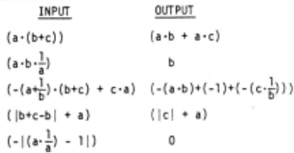
2.4 SIMPLIFY. This is an algebraic simplifica­ tTOn rout1ne which converts algebraic expressions into a canonical form, sorts its terms, and cancels complementary terms of the form (a+(-a)) and (a·l) . It is used in all of our routines a which manipulate algebraic expressions. Such

routines are not new to the literature.

Examples.

3. Limit Heuristic. The limit heuristic rule defined below, in conjunction with the routines described in Section 2, is used to help prove limit theorems. LIMIT-HEURISTIC: When trying to use a hypothesis of the type

(and possibly other hypotheses) to establish a conclusion of the type

first tr! to find a substitution o which will allow B0 to be expressed as a non-trivial com­ bination5 of A0 , (B = K·A + L) o, and then try to establish the three new conclusions :

Such a procedure is valid because if we can find such a a and prove A, B, and C, then we would have

Of course, this is based on the triangle inequal­ ity, and uses the fact that l/2 + l/2 = 1, M·l/M = 1 for M > 0 , etc .

As an example, in proving the theorem that the limit of the product of two functions of real variables is the product of their limits, we find ourselves trying to establish a conclusion of the type

4. The notation B0 denotes the result of ap­ plying the substitution o to B.

5. The routine EXTRACT, described in Section 3.1 below, is used to express Bin terms of A.

Among our hypotheses is

which can be used to help establish (1) (provided that we satisfy the conditions for (2)) . If we apply the limit heuristic to (2) and (1) we find

that fo r o = [x/x']

can be expressed as a combination of

viz . ,

and are able to establ i sh the three subgoals :

Subgoal A follows from the hypothesis

(whi ch also has conditions that must be satis­ fied) . Subgoal B follows from (2), and subgoal C follows from (3).

The complete proof of the limit product theorem is given in Section 5 in great detail. The limit heuristic is used there not only to set up the three subgoals A, B, and C, but also to establish A and C, by proposing further subgoals.

Because the limit heuristic enables our program to prove many theorems about limits, we regard it as a rather interesting trick. But more interesting and important than the fact that it works some problems is the principle behind it . That principle might be stated:

To establish a conclusion C from several hypotheses , among wh i ch is H, force H to contribute all it can towards establishing C and leave a remainder to be established with the help of the other hypotheses .

The value of such a "forcing" technique is twofold . First, if one can truly make H con­ tribute all it can towards C, then His not needed to establish the remainder. That is, a reduction in the number of hypotheses is achie~ while a significant step in the proof is made .

Second, it is implicit in the notion of "force " that certain facts are used to make an i nference in a computational manner. For example, the limit heuristic "uses" many facts about algebra, such as the triangle inequality;

but these facts are used to comoute something, not to make random inferences. This strongly inhibits the generation of subgoals that occurs if one freely permits the application of axioms to his goals . We coiTment further on this "com­ putational" aspect of the limit heuristic in Section 7.

We feel that such a forcing technique has applications in other areas of theorem proving where two or more hypotheses H1, H7 , ..· Hn are needed to establish one conclusion C that cannot be logically divided. In such applications the user must provide a heuristic which will enable the computer to determi ne how to qet a partial result from H1 and leave a reaminder C' to be proved by the other hypotheses .

The limit heuristic uses the routine EXTRACT described below, which in turn uses the simplification routine described in Section 2.

3.1 EXTRACT . If there is a substitution o for which B 0 can be expressed as a non-trival com­ bination of A0 ,

then (EXTRACT A B) returns (K L o), where o is the most general such substitution . Otherwise NIL is returned.

A more precise definition follows the ex­ amples.

Examples. In the following, the symbols x, t, and h represent variables while all other symbols represent constants.

1. (EXTRACT A (K·A+L)) ( K L T) . 6
2. 2 0 (EXTRACT A(t) A(t 0 )) (10[t 0/t]).
3. (EXTRACT (f(x)-L 1 ) (f( x0)+g(xo) - (L 1+L 2))) (1 ( g (X 0 ) - L 2 ) [x ifx]).
4. (EXTRACT (f(x)-L 1) (f(x 0) . g(xo)- L1·L2l = (g(xo) ( L 1 ·g( Xo) - L I ·L2) [x 0/x]).
5. 50 (EXTRACT ( f( X) -L 1) 1 1 7 (nxr- ~ ll

1. (EXTRACT ((x0-a) (x0 2 - a2)) = ((x 0+a) 0 T~

6. Throughout this paper we use the letter "T" to denote both "truth", and the empty sub­ stitution . This reserves "NIL" for denotinq "false".

7. In this example, the second argument i's firstconvertedto(L 1 · 1 -f(x)· 1 ), TTXTT, 1\"XT:r I by use of a least common denominator .

Examples 3, 4, 5 ane useful in proving limit theorems about the sum of two functions, the product of two functions (see Section 5), and the quotient of two functions. Example 6 is used in proving that a differentiable function is continuous.

Suppose there is a substitution o and an expression x such that, A0 and B0 are poly­ nomials in x, and B is linear in x. Then there are expressions a, c, b and d such that x does not occur in c, b, or d, and A0 and B0 can be re­ expnessed as

and (EXTRACT A B) returns the value (Q. (d - Q..:£) o). If no such o and x exist a a then EXTRACT returns NIL.

!· The Implication Method

At the heart of the program is a subroutine called IMPLY whose essential purpose is to handle logical deductions in the predicate cal­ culus . It is a replacement for resolution in [1). We offer here a cursory description of its operation, sufficient to an understanding of the proofs in Section 5.

The operation of IMPLY bears a closer resemblance to the proof techniques of the mathematician than does resolution. In general IMPLY examines the connectives in the formulas, given as arguments to it,and creates one or two subgoals. These subgoals are usually calls to IMPLY with new arguments which are closely related to but simpler than the original argume~ The resulting analysis of the formula to be proved is easy to follow.

This rather natural operation bears some responsibility for the development of the limit heuristic and the other techniques of this paper. In comparing the subgoals called by IMPLY with the methods of proof used in elementary calculus we established new subroutines and subgoals, such as the limit heuristic, sufficient to prove a number of theorems.

The subroutine IMPLY has two arguments:

E (the curnent formula under

examination)

R (a neserve) . Usually E is of the form

The answer to a call to IMPLY is either a sub­ stitution or NIL. The latter indicates failure to establish the subgoal. IMPLY attempts to find and return the most general substitution o such that (R .. E) is true. If o is the empty substitution then°IMPLY returns T.

Table 1 gives rules describing some of the operations of IMPLY. These rules are applied in the order of their occurence in the table; if one fails, the next is tried; if all fail, IMPLY returns NIL. IMPLY returns the value given by the first rule which does not give NIL. In the following we use the shorter notation [E,R) for (IMPLY E R).

This rule is commonly known as backwards chaining.

Table 1 Some of the rules defining IMPLY.

8. When we use an expression like "[A,R] yields o", it is to be understood that we also mean than o is not NIL. (ol o o2) denotes (olo2 1.1 o2).

9. If 4.2 fails but [R .. A 1 v C, NIL] yields o3 ot [(A .. B) 1t.. R · Aql' NIL) y elds r. 3, then IMPLY returns (ol o o3J.

Table 1 (concluded)

Before a formula E is sent to IMPLY it is f i rst converted to a quantifier free form, but without converting it first to prenex normal form. The quantifier free form is achieved by using skolem functions, and is essentially the same as that used by Wang [3] . 11 A call is then made to (IMPLY E NIL).

10. It is possible for IMPLY to yield a substi­ tution which assigns to a variable x more than one value : a/x, b/x, a1b. If this happens and if IMPLY tries to substitute for x in another expression (as it might do using Rule 8.2, 6.2, 2.2, or 4.2), theniMPLY returns NIL .

If Rule 8.2 fails on the ol given by Rule 8. 1 (i.e., if [H + B 1· R] returns NIL), then the program "backs u~" and recomputes 8.1 trying to find anoth~r solution al 1 of [H .. A, R] for which [H + B 1 1 ,R] can succeed. A similar back­ ing up procegaute is used in Rules 2, 4, and 6.

11. Specifically, if "positive" and "negative" are given the meaning as in Wang [3) pp . 9-10, then the elimination of quantifiers consists of deleting each quantifier and variable immediately after it, and replacing each variable v bound by a positive quantifier with a list whose first member is v and whose other members are those var i ables bound by negative quantifiers whose scope includes v. This list which replaces v is

For example the formula

is first converted to the skolem form

where y 0 is a skolem constant and x is a variable , and proved as follows.

1.

(IMPLY (P(y) " (P(x) ... Q(x)) ... Q(y ))

0

1.1 (IMPLY (P(y) ... Q(y ))

(P(x) ... Q(x)))

(by Rule~). This 0 fails.

1.2 (IMPLY ({P{x) ... Q{x)) ... Q{y )) P{y ))

{by Rule 9).

0

1.2 . 1 (IMPLY (Q(x) ... Q(y )) P(y 0 ))

(byRule4.1).

0

This yields a = [y /x] by Rule 1.

0

1. 2. 2 ( IMPLY ( P ( y ) .. P ( x) ) NIL) Ru 1 e 4. 2

o

a

This yields T by Rule 1. So the final answer to 1. is [y /x], and the theorem is proved. 0

For the example

(SOME x (ALLy P(x,y))

.. ALL s (SOME t P{t ,s)))

the skolem form is

(P(x 0 , y) ... P(t, s 0 )) .

A call is made to IMPLY

(IMPLY ( P ( x , y) .. P ( t, s ) ) NIL)

0

0

which yields [x 0 /t, s 0 /y] by Rule 1.

In trying to prove the non-theorem

(ALLy (SOME x P(x, y))

... SO~E t (ALL s P(t, s))),

the skolem form is

(P((x y), y) ... P{t, (s t))

where (x y) and (s t) are skolem expressions . A call to IMPLY

( IMPLY ( P ( ( x y) , y) ... P { t , { s t) ) ) NIL)

fails; Rule 1. cannot be applied because the formulas P{(x y), y) and P(t, (s t)) cannot be unified. A partial unification is given by [(x y)/t], but the resulting pair

P((x y), y), P((x y), (s (xy))) cannot be unified by [(s(x y))/y] because the variable y occurs in (s(x y)).

When attempting to prove an expression E with the help of axioms, A 1 , A 2 , ... ,A, (where all free variables in the A. haOe been universally quantified), a call is ~ade to (IMPLY E 1 NIL) where E' is the skolem form of

In the operations described in Table 3, . a resemblance can be seen between the method of

simply the aoplicatioQ of a sko]em.funct i on to certa,n arguments. W1th no amo1gu1ty, but as an aid to memory, the skolem function is named v.

QED .

o

NIL) 0

Gentzen sequents {cf. Kleene's G3 [4]) and the subgoals which IMPLY sets up. The technique of of finding a most general unifier is the unifica­ tion algorithm of Robinson [2] . On the whole, IMPLY is closer to the system of Prawitz [6] than to resolution .

5. Examples of Computer Proofs.

Here we give excerpts from the proofs of five theorems, which were made by the program PROVER using IMPLY as its principal subroutine. PROVER is explained in [1] and IMPLY is described briefly in Section 4 above, but the reader famil­ iar with Sections 2 and 3 should be able to follow these descriptions with no reference to [1] and little to Section 4.

In order to use the limit heuristic described in Section 3, we must add the following rule to Table 1.

16.

[ ! A I < E' .. I B I < E , R]

If

16 .0 {EXTRACT A B) is {K L o)

and if

{i.e . , {B = K·A + L) 0 ),

16.1 [R -+ { IK! < M) 0

, NIL) yields oll2,

for some variable M! 3 and if

16 .2 [ !AI < E'

!A! < E/2·1'1, R]{ oo ol)e

yields c2, and if

16 .3 [R - {ILl < E/2){

yields c3, cc ol oo2

)' NIL]

then return the value {oo olc o2o c3) 1 "

Also, we need two additional rules for solv­ ing inequalities, one rule for types, and one for equations.

17 .

18.

19.

[H - a < b, R)

{SOLVE< a b)

( {b < c) v {b =

c

c) , R]

0

if there is a substitution for

which {a = a' ) .

[H - A E B, R)

:J

If A has type B then return T.

These five reles are placed at the beginning of Table 1 {Section 4) , in the order 17, 18, 19, 20, 16 .

Also, a provision is made for assigning a type to an expression A when it appears in the form {A c B) or {A < B) in the hypothesis of the theorem being proved . This is accomplished when IMPLY is proving a subgoal of the form [H .. C, R] by replacing H by {SET-TYPE H). Such calls to SET-TYPE need only be made in Rules 5, 10, 13,

12. In case K = 1, Step 16.1 is omitted, and M is set to 1 in 16.2.

13. Misgiven type <0 ·~ > and also M is made an additional argument of all skolem functions which already have at least one argument. 14. In case L = 0, Step 16.3 is omitted.

[a < b - a' < c, R)

and before the first call to IMPLY,. i.e., when new material is added to H. {See Section 2.3). In what follows, R denotes the real numbers, P denotes the positives~ and FRR denotes the tunctions on R to R. We use {Lim f a L) to denote lim f\x) ~ L. The standard definition x-a of 1 i mit is :

{Lim f a L) <->

{a c ~) " { L c ~) " { f c FRR) "

ALL E { 0 < E .. SOME 6 { 0 < 6 "

ALL x { x c ~ I\ x -;. a A I x - a I < c_

- jf{x)- Ll <c) ))

Example 1 {Limit of a product). The program PROVER is given the formula

{Lim fa L 1 A Lim g a L 2

Lim {f·g) a {L 1 ·L 2 )

The definition of limit is used to obtain

{ {a c ~ " L 1 c ~ " f c F RR "

ALL E 1 { 0 < E l .. SOME 0 1 { 0 < 0 1 A

ALL x 1 { x 1 c ~ 1\ x 1 1 a " I x 1 -a ! < 0 1

jf{x 1 ) - L 1 ! < E 1 ))))

{a c ~ " {L,-L 2 ) c ~ A {f·g) c FRR"

ALL E { 0 < E .. SOME 0 { 0 < 0 /\

ALL x { x c ~ " x -;. a 1\ I x -a ! < D

The first three parts of the conclusion, {a c R), {L ·L) c R, and {f·g) c FRR are proved by the progfam 2 using the hypotheses of the theorem and the closure properties of R and FRR . The remainder of the theorem is prepared for IMPLY by replacing (f.g){x) by {f{x)·g{x)) and by eliminating the quantifiers and introduc­ ing skolem expressions.

For readability and brevity, the skolem expressions are abbreviated in the following . Th us x is used in place of (x D), L in place of (L 1 ) , f( x) . in place of (f)((x D)}, And so on. Thus we wr1te the above expression as

But the computer continues to use the full skolem notat i on throughout its proof.

Before we follow the proof procedure for this theorem in great detail, we first sketch the proof that the computer will produce.

Given E > 0, choose M, M', E 1 , and E 2 so that

By hypothesis, there exist D 1 and D 2 such that

0 < D 1 and 0 < D 2 , and for a 11 x, if x ; a and I x - a 1 < min ( D 1 , D 2 ) , then

it fo llows that

So let D be a number such that

If X i S any number such that x 1 a and fx - a) < D , then

and

The key to this proof is the proper selec­ tion of M, M', E , E , and D. The computer makes precisely thes~ same selections through its handling of types .

We now resume the description of the compu­ ter 's procedure in finding its proof. A call is made to

where o. , ~ . and y are given in (ii) above. SET-TYPE is applied to (o. A e), assigning type ~to a, L , L , and type FRR to f and g, and the subfor~ula~ (a c ~) , (L c ~), (L c R), (f E FRR), (g E FRR), are remov~d from(). ~nd e. Rule 5 is applied, converting the formula to

SET-TYPE is applied to the hypothesis; E i s as­ signed type < 0~> and (0 c E) is removed. Rule 8 calls IMPLY on the two formulas

The first call is satisfied by Rule 17, which uses SOLVE < to assign type <0 ®> to D. The second results in an application of Rule 5, so the current subgoal is

SET-TYPE is applied to the hypothesis; xis assigned type R and (x c R) is removed . By Rule 9~ the reserve R is set to

becomes the current goal.

Rule 4 (backward chaining) is now applied . That is, the program tries first to establish the co~cl~sion /f(x) ·g(x)- L 1 ·L 1 1 < E from () . Th1s 1s subgoal (1). When thTs subgoal is es­ tabl i shed, the program tries to satisfy the hypothesis of () , namely subgoal (2) below.

SET-TYPE assigns type < 0 oo >to D 1 and

becomes the current goa 1. (From now on we sha 11 not mention those subgoals which are tried but not established.)

Again the program "cha i ns backward " using Rule 4. The current subgoal becomes (11) and the hypothesis

( x 1 c B. 1\ x 1 ; a 1\ I x 1 - a I < D)

is satisfied later at (12) .

(11) {lf(x 1 )- L 1 1 < E 1 -+

lf(x)·g(x) -L]"L 2 !<E)

The program now tries to apply Rule 16, the limit heuristic . First

(EXTRACT (f(x 1 ) - L 1 ) (f(x) ·g{x) -L 1 ·L 2 ) )

is computed to be ( g(x) (g (x) ·L 1 - L 1 ·L 2 ) o )

where o = [x; x 1 ]. This follows from the equat i on

(f( x) ·g( x) - L 1 .L 2 J =

((g( x) ·(f{x) - L 1 ) + (g(x)·L 1 - L 1 ·L 2 )) . Because the result of the call to EXTRACT is not NIL, Rule 16 is applicable. The program tries to establish the three subgoals (1 11), (112), (113), in accordance with Rules 16.1 , 16 .2, and 16 . 3. The current subgoa l is

where M is a new variable which is assigned type <0 ~ > . (Also M is made an add i tional argument in the skolem expressions (D 1 E 1 ), (D 2 E 2 ), and (x D),

in accordance with Footnote 13 above . Although these new skolem expressions (D 1 E 1 M), (D 2 E 2 M) ,

and (x D M), wi ll not appear in our descriptions ~ince we are abbreviating them to Dl, D2, and x, they nevertheless play a crucial ro e . For ex­ ample, i n Step (111 1) below theM in (x D M) prevents Rule 17 and SOLVE < from ass igning type < lg( x D M)j oc> as the answer to (111 1) . (See Section 2.1 .

By Rule 9, the reserve R is set to ( x ; a /\ I x - a I < D) and

becomes the The current pothesis of current subgoal . Rule 4 is applied . s ubgoa 1 becomes ( 111 1 ) and the hy­ B is satisfied later at (111 2).

(111 1) ( 0 < 02 1\

By Rule 9 the program tries

after assigning type < 0 oo > to o 2 .

Another application of Rule 4 sets up the two subgoals (111 11) and (111 12).

( 111 11 J ( 1 g ( x 2 J - L 2 I < E 2 ..

1 g ( x J 1 < M)

Since (EXTRACT (g(x 2 ) - L 2 ) g(x) ) yields (1 L 2 [x/x 2 ] ) the limit heuristic is applicable to (111 11). Because 1 is returned as the val­ ue of K from EXTRACT, only subgoals (111 111) and (111 112) are tried, i n accordance with Rule 16 . The current subgoal becomes

By Rule 18 , the program tries to establish

The first half of the disjunction is satis ­ fied by a call to (SOLVE< E/ M/2), givi ng type <-oc M/ 2> toE/ . Thus subgoal (111 111) is estab­ lished and the program tries to prove

(111 112) (x ~a) 1\ lx- a ! <D ..

/L 2 1 < M/ 2) .

Rule 17 is applied; (SOLVE < IL 2 / M/2 ) is called, result i ng in the type < 2· L 2 ,oc , for M.

Hence both subgoals of (111 11) are established. The program now returns to the subgoal

(111 12) (x; a /1. lx- a : <D

x 2 £ B_ /1. x 2 ; a /\ I x 2 - a ! < 0 2 ) c , where o = [x;x 2 ] . That is

( x i a "

I x - a l <D

X c R 1\. X ; a 1\ X - a < 0 2 ).

This subgoal is established by several subcal l s . The conclus i on (x c R) follows since x has t ype B_. (x ; a) occurs in the hypothes i s . And f inally

is established through Rules 18, 17, and a ca ll to SOLVE ·. As a result , the type of D is changed to <O c 2 > .

( 111 2)

(X ; a " i x - a , ' D - 0 < E 2 )

is establ i shed by Rule 17 . SOLVE( types E 2 as <0 M/2 >. Reca 11 that E was given type < - ~ M/2> at (111 111 2 ) . Thus both sub~ goals of (111) have been established and the program returns to the second subgoal of the first use of the limit heur istic

This subgoal is quickly estab l ished using Rules 17, 18 and(SOLVE · E 1 E/2M), whi ch ass i gns type ·-·· E/2M> to E .

The third subgoal 1 of the first use of the l imit heuristic is

( 113) ( f 1\ x ; a 1\ !x - a < D

By Rule 9, the reserve R is set to ( x "I a 1\ :x - a ; . D) ' and the current subgoal becomes

The program chains backward twice.

yields (L 0 T), the limit heuristic is again applicabl~, and subgoals (113 111), (113 112), and (113 113) are tried .

becomes the current subgoal, where M' is a new variable of type <0 ~> . This goal is established byassigningtype <; L 1 1 ·> toM',byRulel7.

~ lg(x) - L I < (E/2)/2·M' ) This subgoal is established 2 by use of Rules 17, 18, and a call to (SOLVE < E E/4 ·M'). E is retyped as (intersection <0 M/2 2 > <- ~ E/4 ·M' 2 > ) . Recall that E had been given type <0 M/2 > to establish (llt 2). Since the program does not know which of M/2 and E/4·M' is the smaller, the intersection is given as the answer, after it has checked that the intersection is non-empty.

The formula

is the last subgoal of the last use of the limit heuristic . It is satisfied since E already has type <0 ~> .

The program now returns to

i s the same as (111 2).

All of the subgoals of the first application of the limit heuristic at (11) have been estab­ lished, giving as an answer to (11) the substitu­ tion a = [x/x 1 , x/x 2 ].

The program now tries to satisfy

The substitution [x;x 1 ] establishes the first two parts of the conclusion. To prove the third part, the program tries

which results in the retyping of D as (intersect i on <0 D 7 > < -~ D 1 > ). Recall that D previously had type <0 D 2 >.

Finally th~ subgoal

is established by Rule 17 and a call to (SOLVE < 0 E 1 ) which retypes E 1 as <0 E/2 ·M>. E 1 previo~sly had type <-~ E/2·M>. QED.

The proof is complete. We list here the final types assigned to the variables. Note that the program has made just those "choices" describ­ ed in the sketch of the proof which was given earlier.

This proof may seem long and drawn out but these are essentially the steps a human prover would have to follow in finding and exhibiting a proof.

In the following examples we proceed directly to skolem form and consider only the proof of the main concl usions . Many steps in each proof are omitted . Rule reference numbers are sometimes given to the right of formulas along with new type assignments .

Example 2. (Composite continuous function theorem) .

1. (g is continuous at a)

In 3. the variables are E 1 , x 1 , E 2 , x 2 , D, and the skolem expressions are (D 1 E 1 ), (D 2 E 2 ), (E), (x D), (a), etc.

CURRENT SUBGOAL

1. (H3ls ~ 0 < D)
2. (SOLVE< 0 D)

RULE NO. and NEW TYPE ASSIGNMENTS

D <0 ~ >

15. The notation Hi is used to denote the hypothesis of Step 1.

1. { I f{x 2 ) - f(g{a)) I ~ E 2 ... lf(g(x)) - f{g(a)) I <E)
2. (E 2 < E V E 2 = E) 18
3. {SOLVE< E 2 E) 7. 17 E <-oc E> a condftion from Step 7. 10. {H 6 ... 0 < E 2 ),
4. (SOLVE< 0 E 2 ) 17 E 2 <0 E>
5. (H 6 .,. x 2 c ~ A x 2 fa 1\ lx 2 - a l <D 2 ) 0 , where o = [g{x)tx 2 ] . A condition from Step 7
6. 13 . (H 6 ... l g(x) - a! < D 2 ) 8
7. ( 1 g ( x 1 ) - g {a) ~ < E l ) ... Jg{x) - g(a) ! < D 2 )
8. {SOLVE < E 1 D 2 ) 18, 17, c = [xtx 1 ] El <-~ D2>
9. {H 6 ... l x - a I < D 1 ) . A condition from Step 14 .

Example 3. (Differentiable functions are

1. {Derivative fa F' ... Continuous fa)
2. (Lim q 0 F' Lim fa f(a) ), where q{h) is the difference quotient f(a+h) - f{a) h

In 3. the variables are E 1 , h, D, and the skolem expressions are (D 1 E 1 ), {E), {x D) ,(F') ,etc

continuous).

The limit heuristic (Rule 16) is applied, (EXTRACT (f(a+h) - f{a)- F') {f(x)- f{a)) h

yi e 1 ds { { x - a)

{ x - a) · F' o) , where

o = [{x - a)/h) .

10 .

11.

12.

(SOLVE< E 1 E/2·M)

{H 4 .. l {x- a)·F' I < E/2)

{ !x-a i< D ..

18, 17

E 1 <- "' E/2M>

Rule 16 . 3

l{x-a)·F' I< E/2)

The limit heuristic yields {F' 0 T) ·. is again used, EXTRACT

1. M <IF' ! «> ( !x- a l < D .,. lx- a l < E/4·M') , 16 .2 etc.
2. 16 . {x fa A !x- a ! < D .. h ( ~ /\ h f 0 1\ ! h ! < Dl ) ;J. 4. 2 a condition for Step 5. a = [( x - a) / h).
3. 8 {H 16 .. {x- a) E ~) True by Rule 19 since both x and a have type ~·
4. 18 . (x ; a ... x - a ; 0), from Step 16. 8, 9

1. (SOLVE= {x - a - 0) {x - a) ) 20, TRUE

21.

( lx-a i <D ... lx-a !

8

from Step 16

1. {SOLVE< . D D 1 ) 17. 18 D is assigned type (intersection <0 E/4·M' > <- "' D 1 > ). QED.

1. { f = >. X (x· x) .. Lim f a {a · a)) 2. (0 < E ... (0 < D 1\ {x c R 1\ X f a 1\ l x - a! < D l x·x- a·a l < E)))
2. In 2. Dis a variable and {E), { x D), and {a) are skolem expressions.

First SET-TYPE assigns type <0 oo> to E. Then

1. {0 < D) Rule 8. 1

1. (SOLVE . 0 D)
2. D -o 5. (X ~ a /\ i X - a ' < D 'x·x - a·a ! < E) 8. 2,5 from Step 2. X is assigned type R.

6. ( :X - a ; < D lx·x - a·a : < E)

Rule 17

9

The limit heuristic is used, (EXT~ACT (x-a) (x-x- a·a) ) yields ( (x+a) 0 T).

7.

(H 5 - !x+a : < M)

The limit heuristic is used again,

(EXTRACT (x-a) (x+a)) yields (1 2·a T) .

8. ( I x - a 1 < D - i x - a , · M/ 2)

16.1

16 . 1

from Step 7.

9.

(SOLVE< D M/ 2)

10. (H 7 - '2·a : < M/2)

from Step 7.

11. (SOLVE·

i2·a i M/ 2)

12. ( :x- a : < D -

1 x-

· from Step 6.

13 . (SOLVE < D E/2 ·M)

18,

<0 M/2 >

16.2

17

<2 · '2·a

16.2

17

D is assigned type

{in~ersection ·0 M/ 2> ·-· E/ 2·M· ) . QED.

Example 5. (Limit of a quotient) .

The proof of this example is not complete .

1.

(Lim fa L /\ L ~ 0

Lim (1/f) a (1/L)).

2.

( 0 · E l - ( 0 < D 1 /\

( x 1 ;: R 11 x 1 ~ a 1\ ! x 1 - a ; · D 1

. f(x 1 )- L! · E 1 ) ))

/\ L ~ 0

(0 < E -

(0 < D 1\

(x ;: R 11 x ~a /1 : x - a l · D

I 1

1

!nxT- r : · Elll

: 1

3. ( f(x 1 ) - L: < E 1

1 '

if\xT- fi < E)

The limit heuristic (Rule 16) is applied,

(EXTRACT (f(x 1 ) -L) (rfxr- tll yields (-L~

0 ~ ).where : = [x;x 1 ] .

We are required by Rule 16 to establish the subgoal s

and

(2) ( if (x)- L! < E 1

if(x)- L! < Ef2 ·M),16.2

Subgoal (2) is easily established by assign­ ing type < -oo E/2 ·M> to E 1 , but (1) presents difficulty. In fact the program is unable to give a proof of (1) without some axioms or a change in t he program. See Section 7 for further comments on this example.

17

'L>

D

M

a ; ·E/2 ·M)

6· Resolution.

In this section we show how the limit heur­ istic and the theory of types explained above can be used in resolution based programs . This is done by giving some additional rules for resolu­ tion. These are:

6. 1 SET-TYPE Rule .

For each unit clause of the form (x . A). where x is a skolem expression which does not oc­ cur in a, assign the type A to x. Also for each unit clause of the form (x · a), where xis a skolem function which does not occur in a, assign the type <- · a> to x. Similarly for unit clauses of the form (b · x) assign type ·b ·· to x. In each of these cases, remove the unit clause. If x already has a type B and we are try­ ing to assign it a new type A, then assign the type (>~n B) if it is non-empty; if (A'"' B) is empty, add the empty clause (i.e., the proof is finished); if it cannot be determined whether (An B) is empty, leave the original type as is and do not remove the unit clause . This SET-TYPE rule need only b~applied at the beginning and after each new unit clause is generated .

6. 2 MEMBFR Rule.

For a clause of the form

(1 ) if x has type A then add D to the list of clauses, (2) if xis a variable and x does not occur in A, then assign the type A to x and add D to the list of clauses.

6. 3 TRANSITIVE Rule .

When attempting to resolve two clauses of the form ((a · b) v A) and ((a' i c) v B), where a =a' for some substitution o , if (SOLVE< 0 b c) 0 yields o ', then add the resolvent 0

(A v B) ,e to the list of clauses. G O O

6.4 SOLVE· Rule.

For a clause of the form

0 v (A I B),

if (SOLVE< A B) yields the value : , to the list of clauses . then add D a

6.5 SUBTRACTION Rule .

When attempting to resolve two clauses of the

form

if (SOLVE= (a-c) (b-d) ) yields value o, then add (A vB) to the list of clauses. 0

6.6 ~OLVE= Rule.

For a claus~ cf the form

D v (A ~ B),

if (SOLVE=~ B) yields the value _, to the list of clauses. then add D 0

Before going to our limit heuristic rule; we give some examples using the above six rules.

Example 1. (0 < a Clauses ~ SOME x ( 0 < x A x < a) ) . Clause Rule and Reference new Type Assignments l. 0 < ao } From Theorem 2. 0 I X V X f. a 0 3 . SET-TYPE ao <0 co> 4. X f. ao 2 SOLVE< X <0 co> 5. 0 4 SOLVE< X <0 ao>· We could have removed X f. a 0 first, 4. 0 f. X 2 SOLVE< X < -~ ao> 5. 0 4 SOLVE< X <0 ao> Example 2. (0 < 01 " 0 < o2 SOME 0 (0 < 0 " 0 < o 1 " 0 < 0 2 )) l. 0 < 01 2. 0 < 02 } F'Om 3. 0 f. 0 v 0 f. o 1 v 0 f. 02 Theorem 4. SET-TYPE 01 <0 ~> 5. 2 SET-TYPE 02 <0 ~> 6. 0 f. 0 1 v 0 f. 0 2 3 SOLVE < 0 <0 «-> 7 . 0 f. 0 2 6 SOLVE< o <O o 1 , 8. 0 7 SOLVE< 0 At Steps 7 that o 1 and (intersection <0 01 > <0 02 > and 8 SOLVE < required the knowledge 0 2 both had type <0 ~>. Example 3. l. X t p 2. X £ N 3 . X = X 4. 5. 0 Example 4. (x c !:_ " x t !:!_ ~ x 'f x) } From Theorem (x is a skolem constant) 2 SET-TYPE X <0 " ·> SET-TYPE (0 < a A 0 < b ~ (SOME z (O<Z A (c<Z C<a) A (d<Z ~ d ~b))) l. 0 < a 2. 0 < b lf. From Theorem. a, b, c, d are skolem constants. z is a variable .

(intersection <0 b,.O a>) .

By ordinary resolution Example 4 would re­ quire at least two axioms,

Al.

(0 < a "' 0 < b

and a long and difficult sequence of resolution steps . This very example occurs as a disguised part of the proofs of most of the limit theorems , and therefore it is important to have an easy proof for it requiring no axioms.

We now give the LJMJT-HEURJSTJC Rule .

6.7 LIMIT-HEURISTIC Rule.

When attempting to resolve two clauses of the form

try to find a substitution ,, which will allow B to be expressed as a non-trivial combination of A,

and, if this is possible for some substitution .·; , then add the following new "resolvent" clause to the clause list

where M is a new variable with type <0 .,··. The first part of 6.7 can be done by {EXTRACT A B) . See Section 3.1. EXTRACT produc­ es the desired K, L, and :, where - is the most general such substitution .

16. Also the variable M is made an additional argument of all skolem functions appearing in (1) which already have at least one argument.

Example 5. Given the clauses

where E 1 , E 2 , x 1 , x 2 , are variables, and E, E 1 , E 2 each has type <0 ®>,

Rule 6.7 is used on clauses 1 and 3; (EXTRACT (f(x 1 )-L 1 ) (f(x)+g(x)-L 1 -L 2 ) ) yields {1 (g(x)- L 2 ) [x/x 1 ]) (see Section 3.1); and the following resolvent is produced

Example 6. (From the theorem that a function hav­ ing a derivative at a point is continuous there). Given the clauses

where h, O,and E 1 are variables, and the other terms have type R.

In attempting-to resolve 1 and 2, the limit heuristic Rule 6.7 employs EXTRACT to express

as

where ., is the substitution [(x-a)/h]. It there­ fore produces the resolvent

where M is a new variable of type <0 ~> Rule 6.3 applied to 3 and 4 gives

and 0 is assigned type <- " M·. Rule 6.3 applied t o 1 and 5 gives

and E 1 is assigned type <- ·· E/2-M>. Again the limit heuristic Rule 6. 7 is used on c lauses 3 and 6. EXTRACT yields

and the new clause

is produced, where M 1 is a new variable of type <0 ~>. Rule 6.4 is applied to 7 to obtain

and M' is assigned type <IF' I ®>, Finally, Rule 6.3 is applied to 3 and 8 to yield 0. QED.

This final step also assigned to 0 the type {intersection <-® E/4·M'> <0 M>).

Ordinary resolution would require several axioms for this nroof and a very long deduction.

The clause (1) which is added by the Limit­ heuristic Rule 6.7 can be thought of as a kind of "catalyst" clause, because it speeds up the der­ ivation of 0 (without the necessity for addition­ al axioms). It might be useful to produce similar catalyst clauses in other situations where diffi­ cult proofs are required.

7. Corrments.

One remark is that, except for the example on quotients, (mentioned again below) these limit theorems were proved without the inclusion of axioms (reference theorems). This is desirable because,for most automatic theorem proving pro­ grams, the axioms have to be selected by humans for each theorem being proved. Of course, we had to include the limit heuristic itself which acts like some axioms, but it does not hinder the proof of other theorems not requiring it, because it does not release its action unless its need is detected. This is in the spirit of the "Big Switch" mentioned by Newall, Feigenbaum, and

others.

It was surprising to us that so many theorems would follow from one heuristic . Will this happen in other areas of mathematics? Can we provide a series of heuristics with big switches which will handle many areas of mathematics without excess­ ive irrelevant co~puting? We doubt that it can be so simple, but nevertheless feel that such heuristics should be sought for other areas of mathematics . The success of such a collection of heuristics will depend in great part on the cleverness of the overseer program which directs the use of these heuristics . Hewitt's program­ ming language PLANNER [5] or the Stanford Research Institute language QA4 might be well suited for writing such overseer programs, or for improving existing ones .

CALCULATE VERSUS PROVE

One thing that contributed to the success of this effort was the use of the routines SOLVE<, SOLVE=, and SIMPLIFY. The point is that these routines were used to calculate something rather than prove something. Since proving is inherent­ ly harder than calculation, we feel that such routines should be employed as much as possible. Think how difficult it would be in our proofs to employ a set of algebraic simplification axioms in place of t he routine SIMPLIFY. Or suppose that instead of us ing EXTRACT to give a decomposition, we tried to prove that such a decomposition exists . This suggests that more use ought to be made of calculation procedures within the proving mechan­ isms of automatic theorem provers . For example , The un i fication algorithm is such an example, and it revolutionized automatic theorem proving when J . A. Robinson def i ned its role in resolution. A source of power to a mathematician is his ab i l­ ity to leave to calculation those things that can be calculated and thereby free his mind for the harder task of finding inferences .

in proving theorems about	we might calculate
derivatives	1 imi ts
1 i mi ts	solutions to equations and inequalities
differential equations	derivatives
real functions	solutions to equations
measure theory	that two sets are equal
algebraic topology	group theoretic results
anything	a most general unifier

MEMBERSHIP TYPES

The use of membership types also helped con­ siderably in proving these limit theorems. It is as if in proving,

we first find A, the set of all x for which P(x) is true and assign A as the type of x, and then find B the set of all x for which Q(x) is true and if (AI'\B) is not empty, assign it as the type of x, and declare (2) to be true. This allows a maximum amount of freedom in the proving of Q(x) after P(x) has been proved; indeed x remains a variable, even though restricted, in the proof of Q(x) . This idea is somewhat related to constraint methods used by Fikes in [7].

This procedure worked well in our examples because linear inequalities are so easy to solve . We do not recommend that such a procedure should be used in all other situations, when theorems of type (2) are being proved, because it may be too difficult (or unnecessary) to solve for A, the set of all x for which P(x) is true, before prov­ ing Q(x). We do suggest however that a procedure be fullowed that leaves x as a variable, though restricted, after P(x) has been proved and while Q(x) is being proved . Type theory might help attain such an objective .

Our present program will not prove limit theorems involving quotients, such as

without the help of some axioms (see Example 5, Section 5). However, no axioms are needed for the proof of (3) if we add another heuristic to the program which is similar to the limit heuristic, but which is based upon the inequality ix: - ly ' ~ ·x- y ;

instead of the triangle inequality

upon which the limit heuristic is based. In fa ct, it might be desirable to develop a more genera l heuristic, which not only encompasses both ideas, but also tries to attain such objectives as bounding an expression, e .g. ,

and making an expression small, e.g.,

Finally, it should be mentioned that t he routines descr i bed in Section 2 are meant for general use in analysis and not just as an ai d i n proving limit theorems. It is hoped that routines of this kind can be used to make an analysis prover in which relatively simple heurist i cs can be added for great effect .

1. Acknowledgement. The work reported herein was conducted at the Artificial Intelligence Lab­ oratory, a Massachusetts Institute of Technology research program supported by the Advanced Re­ search Projects Agency of the Department of De­ fence, and was monitored by the Office of Naval Research under Contract Number N00014-70-A-03620002, and was also supported by National Inst i ­ tutes of Health Grant GM 15769-03 .

References .

1. W. W. Bledsoe, "Splitting and Reduction Heuristics in Automatic Theorem Proving," Artificial Intelligence£ (1971) pp 55- 77 .
2. J . A. Robinson, "A Machine-Oriented Log i c Based on the Resolution Princ i ple ," Jou r . ACM 12 (January 1965) pp.23-41. --
3. Hac Wang, "Toward Mechanical Mathematics, " ~Jour . Res . Dev . , 4, pp. 2-22 .
4. S. C. Kl eene, Introduction to Metamathemat i cs , D. van Nostrand, New York: 1952 .
5. Carl Hewitt, "Planner," M.l. T A. I. Memo No. 168, August 1970.
6. Dag Prawi tz, "An Improved Proof Procedure ," Theoria, 26, pp . 102-39 .
7. R. E. Fikes, "REF-ARF : a system for solving problems stated as procedures, " Artificial Intelligence l (1970) pp.27-120 .