
Solving Problems by Formula Manipulation in Logic and Linear Inequalities
Proceedings of the Second International Joint Conference on Artificial Intelligence. Pages 553-558.
© 1971 International Joint Conferences on Artificial Intelligence
Abstract
Using formal logic, many problems from the g eneral area of linear inequalities can be exp ress ed in the elementary theory of addition on the real numbers (EAR) . We describe a method for e l i mi nat i ng quantifiers i n EAR which has been pr ogr ammed and demonstrate its usefulness in s ol ving some problems related to linear prog ra mmi ng. I n the area of mechanical mathematics this kind of app r oach has been neglected in favor of more g eneralized methods based on Herbrand expa n sio n. However, in a restricted area, such as l i nea r inequalities, the use of these specialized me t hod s can increase efficiency by several orders of ma g nitude ov er an axiomatic Herbrand approach, and ma ke p ra c tical problems accessible.
- Chang, C.L.: Fuzzy Algebras, Fuzzy Functions, and Their Application to Function Approxima- tion. Heuristics Laboratory Report, Division of Computer Research and Technology, N.I.H., July, 1970.
- Collins, G.E.: Tarski's Decision Method for Elementary Algebra. Summer Institute for Symbolic Logic. Cornell University, 1957.
- Gass, S.I.: Linear Programming. Third Edi- tion, McGraw-Hill, 1969 .
- Hodes, L.: Dense Linear Order and Linear In- equalities. IBM Research Report RC-908, 1963.
- Hodes, L.: Programming Languages, Logic and Cooperative Games. Presented at Symposium for Symbolic and Algebraic Manipulation, March, 1966. Abstract in Comm. of ACM, August, 1966.
- McCarthy, J. et.al.: LISP 1 . 5 Programmer's Manual, M. I.T., 1963.
- Rogers, H.: An Example in Mathematical Logic. Mathematical Monthly, November,l963.
- Tarski, A.: A Decision Method for Elementary Algebra and Geometry. Second Edition, Berkeley and Los Angeles, 1951.
- Waugh, F.V.: The Minimum-Cost Dairy Feed. Journ~l of Farm Economics, August, 1951.
References were extracted automatically from the PDF and may contain errors.
Full text extracted automatically from the PDF; figures, tables and equations may differ. The PDF is the version of record.
SOLVING PROBLEMS BY FORMULA MANIPULATION IN LOGIC AND LINEAR INEQUALITIES Louis Hodes
National Institutes of Health Bethesda, Maryland U.S.A.
Abstract
Using formal logic, many problems from the general area of linear inequalities can be ex press ed in the elementary theory of addition on the real numbers (EAR) . We describe a method for el iminat i ng quantifiers i n EAR which has been pr ogr ammed and demonstrate its usefulness in solving some problems related to linear pro grammi ng.
In the area of mechanical mathematics this kind of appr oach has been neglected in favor of more generalized methods based on Herbrand ex pansion. However, in a restricted area, such as l i near inequalities, the use of these specialized me t hods can increase efficiency by several orders of magnitude over an axiomatic Herbrand approach, and make prac tical problems accessible.
l. Int r oduc tion
As is common in artificial intelligence, the work r eported here is of an interdisciplinary natur e . It involves mathemati cal logic, linear inequalities, and symbolic mathematics on a com put er.
For the sake of argument, let us distinguish two kinds of workers in the area of linear in equa l i ties. There is the theoretician, who is deve l oping new methods and discovering new theo rems . Then there is the~. who is faced with a pract ical problem which can be expressed in some way at least piecewise linearly. As a s imp le-minded distinction between the theoretician and t he user we can say that the latter is in t er es ted in questions involving a fixed number of va r i ables, while the former is concerned with ques tions involving an arbitrary number of var iabl es . Using terminology from logic to be made mo re precise below this means that the user i s generally working within the elementary theor y of addition on the reals while the theo retician i s generally working on a higher level.
In this paper we are concerned mainly with the user. at the stage where he has formulated his prob l em in symbolic terms. This may or may not be the first stage in formulating the prob l em. For example, he may first have developed a mode l as a mathematical ideal i zation of his pr oblem. Indeed, if he is very lucky, the model may be of a standard type, for example, flow networ ks, f or whi ch there are known efficient sol ution me thods . In that case he would bypass
a symbolic f ormulation.
Suppose, now, in one way or another the user has arrived at a symbolic formulation of the problem. We assume that the size of the problem is such that he would want to use a computer. Again, he may have a perfectly standard problem such as to find a solution to a set of simulta neous inequalities. Then he can use the relaxa tion method or another numerical approach. Or , if he can formulate his problem as an optimiza tion problem, he may conveniently be able to ex press it in linear programming format and use
the famous simplex algorithm.
Problems can arise, however, which do not fit too easily into the standard molds. Furthermore, one may require a solution in symbolic form. For example in n-person game theory the set of solu tions can be described as a union of convex poly hedra, each of which is an intersection of half spaces, represented by linear inequalities.
Using formal logic one can often represent one's problem conveniently in the lower predi cate calculus under the interpretation of addi tion on the real numbers. In that case, there are simple methods for eliminating quantifiers and s implifying expressions, often resulting in the solution of various problems. Such methods were first programmed by the author at IBM in 1962 (4) and further elaborated with a game theory application (5). Since then some modifi cations and improvements have been made. The complete methods are described here since the earlier papers were never formally published.
Although the author has been addressing him self to workers in linear inequalities, the work reported here may also be categorized as mechan ical mathematics or equivalently applied logic on computers. In this field such work has been neglected in favor of more generalized methods based on Herbrand expansion. The effort on these general methods is, of course, worthwhile and productive, but the neglect is unfortunate since restricted specific theories (like addi tion on the real numbers) often allow the use of direct, specialized methods which increase effi c iency by several orders of magnitude over an axiomatic Herbrand approach.
2. EAR
We now describe the elementary theory of addition on the reals (EAR), or, more precisely , the elementary theory of ordered dense Abelian groups without endpoints. "Elementary" means that all formulas in EAR belong to the lower predicate calculus, i.e., quantification occurs only over variable symbols, and not, for example, over sets of variables. The formulas in EAR, to be defined more precisely below, are just those formulas of the lower predicate calculus with two binary predicates, < and =, the opera
tor+, and at least two constant symbols,
0 and 1.
We refer the uninitiated reader to Rogers' (7) expository paper which, without presupposing any knowledge of formal logic, develops the elementary theory of dense linear order together with a method due to Langford for deciding sen tences within that theory. This method extends to EAR, as pointed out to me by A. Robinson, and is described below. EAR has an unlimited set of variable symbols, x,y,z,x 1 ,y 1 ,z 1 , ... , and real numbers as constant symbols, of which we will need only 0 and 1.
A~ in EAR is either a constant symbol or a variable symbol or of the form t 1 + ··· + tn' where the ti, 1 ~ i ~ n, are terms. These are the only terms.
We write x + ... + x, n times, as nx and l + ... + 1, n times, as n, so the following are examples of terms.
- 2x + 3y + x
- 4 + x 9
Using the commutativity of addition we see that there is a canonical form for terms where each variable symbol appears once. Thus, example (1) above could be written 3x + 3y.
An atomi c formula, or atom, is any expression of the form t 1 · t 2 or of the form t 1 < t 2 , where t 1 and t 2 are terms. There is a canonical form for atoms where each variable symbol appears on at most one side of any atom. For example 3x + 3y < 2x would be written x + 3y < 0. We also allow two constant atoms: TRUE and FALSE.
Atoms are the simplest formulas. Non-atomic formulas are built from atoms by means of the propositional connectives; negation,·-, , "and", &, 11 or", V, "implies~~,-+, "if and only if",<te+, as well as the universal and existential quanti fiers, "for all x", ( 'rl x), and "there is an x such that", ( Jx), where x is any variable symbol.
Examples of formulas are:
- X < y V X = y V y < X
- (jx) (x < y & 2y < x + 5)
- ('tjx) c]x)l2x+y< 0
Formally, we say that an atom is a formula and if f 1 and f 2 are formulas then
-,f 1' (f 1 [, f 2). (f 1 v f 2). (f 1 -+ f 2). Cf 1 ~f 2 ), (\;;fx) f 1 , C3 x) f 1 are all formulas. Every formula is so derived. We delete paren theses to improve readability, being careful not to introduce undesirable ambiguities. Example (1)
above illustrates desirable ambiguity.
For convenience, we us~ t 1 ~ t 2 as an abbre viation of, t 1 < t 2 ·
As a further example of a formula in EAR we represent the statement that ~he real numbers x 1 , ··· , xn minimize the sum r ci xi subject to 1
the conditions
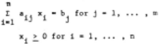
This is a statement of the linear programmin~ problem, and says that x 1 , ... , xn yield an optimal solution. We assume, for simplicity, that the aij' bj and ci are all integers.
We allow the use of the minus sign by con sidering any occurrence .of -tin an atom as a convenient notation for +t on the opposite side of the atom.
The linear programming problem is stated in EAR as follows:
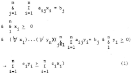
From the point of view of people working in linear inequalities the most novel feature of EAR is the formal use of quantifiers. In fact, the elimination of quantifiers, together with their bound variables, is the main content of the algorithm described below.
3. A Decision Algorithm for EAR
Suppose F(x 1 , ··· , xn) is a formula in EAR in which x 1 , ... , xn are the only free (not quantified) variables. Then the following algorithm yields a quantifier-free formula G(x 1 , ·.· , xn) in which x 1 , ··. , xn are the only variables, with the following property. Let a 1 , ..· , an be any n real numbers. Then F(a 1 , ·. .. , an) and G(a 1 , ·.· , an) are equiv alent in the sense that they are both true or are both false. For example, if F( x) i s t he formula ( ] y) (y < x + 4 & 2x < y + 5) then G(x) would be the formula x < 9.
Since EAR is a subset of elementary algebra, Tarski's algorithm (8) provides a method for elim inating quantifiers. When applied to formulas in EAR, however, Tarski's method is exceedingly cum bersome. Furthermore, no one has reported a com puter program for any algorithm to eliminate quan tifiers in elementary algebra except for some be ginnings in that direction by Collins (2). On the other hand, EAR has a simple method and seems to be in the unique position of having such a simple algorithm along with a wide range of application.
The elimination of quantifiers is achieved by systematically replacing selected subformulas by equivalent formulas. The equivalence may be pure ly logical or may be a property of +, ·, < in the reals, as we used, for example, in establishing a canonical form for atoms.
~· If F(x 1 , ... , xn) is quantifier-free, let G ~F. Otherwise, choose a subformula of the form Cj y) f (x 1 , ... , xn' y) where f is quantifier-free, i.e., ( J y) is an innermost exis
tential quantifier . If all innermost quantifiers are universal quantifiers then use the identity ( V x) g := I (] x) 1 g, so that ( J x) -, g yields the required sub formula ( 3 x) f, with f = J g.
~· We use steps 3-8 to find a quantifier
free formula g(x 1 , ... , xn) equivalent to C]y) f Cx 1 , ... , xn' y). We replace C]y) f by g in F, then return to Step 1.
~· Eliminate all occurrences of equivalence, (~), and implication, (-.) in the formula ( J y)f by the use of identities
~· The only connectives in f are & , V,) . Use the identities
to eliminate all occurrences of negation save those appearing directly before atoms.
~· The remaining negations are eliminated by using the mathematical identities:
Call the new formula ( 3 y) f.
~· Now f has connectives &, V only. Use the distributive law
f 1 & (f 2 V f 3 ) : (f 1 & f 2 ) V (f 1 & f 3 ) to expand f into disjunctive normal form
where each fi is a conjunction of atoms .
lli.l!...l· The existential quantifier dis tributes over disjunction. So ( J y) f - ( 3y) fl v ... v f n
Each fi can be written f' & f" where f' is a i i i (possibly empty) conjunction of all the atoms which contai~ y. Since f~ doesn't contain y,
~· We must now eliminate the quantifier from each formula ( 3 y) f ~. Each such formula must be of the form
For 1 < i~n,ji> 0 is the number of atoms of the type tl · t 2 and ki is the number of atoms of the type tl < t2. We can assume
ji + ki > 0, i.e., f~ is non-empty. In each atom y appears on the right or on the left, but not both, since the atoms are in canonical form.
We now consider the case ji > 0, i.e., there is at least one equality. If ji · 1 and ki · 0 then we replace C3y) (t(i) · s(i)) by the 1 1 constant atom TRUE . Otherwise, we solve ( i) ( i) t 1 · s 1 for y and substitute this expression for y in the remaining ji + ki -1 atoms. Let gi be the conjunction of these ji + ki -1 atoms, restored to canonical form. We replace ( :;J y) f 1 by gi, thereby eliminating the quantifier.
Now we consider the case ji · 0. We have <3 y) f~ of the form
Suppose y appears always on the right, i.e.,
(i) in every r , 1 < p - Then we replace (~ y) f~ by TRUE. Similarly, if y appears always (i) on the left, i.e., in every qp , 1 ~ p ~ ki, we replace <;3 y) f~ by TRUE.
In the remaining case, for each m, p such that y occurs on opposite sides in the atoms Q(i)< r(i) and q(i) < r(i) we eliminate y from "Ill m p p the pair of inequalities by forming the weighted sum, 1£). Each such m, p pair forms a new in equality and finally we get

Note: Let Ci be the coefficient of yin the ith inequality, i · 1,2. Then the weighted sum is c2 times the first inequality added to cl times the second inequality. In the resultant inequal ity ~ has coefficient c 1 c 2 on both sides and thu~ vanishes.
From Step 8 we return to Step 2 to complete the algorithm.
To see that Step 8 always produces an ·equiv alent formula we first maintain that in the case ji > 0, i.e. there is at least one equality, the equivalence is obvious. When j. · 0 then each atomic formula q(i)< r(i~ 1 < ~ < ki, by mathep p - matical identity, corresponds to a linear inequal ity y < f (z 1 , ... ,z ) (or f (z 1 , .·. ,z ) < y, dep v p v pending on which side of the atomic formula y appears) where f is a linear form and z 1 , ··· ,z p v
are all the variables occurring in formula f~ excluding y. We separate the atomic formulas into two sets, corresponding to inequalities {f (z 1 , ... ,z ) ~ y} and {y c f (z 1 , ··· ,z )} where m v p v the respective index sets s 1 and s 2 , where m ranges over s 1 , p ranges over s 2 , form a partition of {l, ··· ,ki}. If y appears on the same side in every atom then either s 1 or s 2 is empty and (] y)f~ can be satisfied for any z 1 , ... ,zv by a sufficiently small y if s 1 is empty or a suffi ciently large y if s 2 is empty. Therefore the algorithm replaces ( 3 y) f ~ by TRUE.
In the remaining case, the algorithm, by taking weighted sums, produces a conjunction corresponding to the simultaneous inequalities f (z 1 , ... ,z ) < f (z 1 , ... ,z ) for all m & s 1 and m v p v all p £ s 2 , To show equivalence we first notice that for any z 1 , .·· ,zv if there is a y satisfying f~ then for each pair m,p there are fm(z 1 , ... ,zv) < y andy< fp(z 1 , .·· ,zv). Hence f (z 1 , ... ,z) < f (z 1 , ·.. ,z ). In the other m v p v Jirection, for any z 1 , ..· ,zv' if all fm(z 1 , ... ,zv), m £ s 1 are less than all fp(z 1 , ... ,zv), p £ s2 then there is a y between them by the denseness of the ordering. Thus (] y)f~ holds.
We can make two observations before giving some examples of the algorithm.
1. If the original formula were closed, i.e., all its variables were quantified, then the al gorithm produces a quantifier-free formula with no variables. In that case the only atoms are of the form 0 < 0, 0 · 0, 0 < n, n < 0, 0 · n, n = 0. These can be replaced by the constant atoms FALSE, TRUE, TRUE, FALSE, FALSE, FALSE, respectively. Then the propositional identities TRUE & FALSE : FALSE, etc., can be repeatedly used as the last step of the algorithm to comp plete the reduction of the formula to a single atom, either TRUE or FALSE. Such an extended algorithm provides a decision procedure for EAR, i.e., a method for determining the truth or falsity of any sentence expressible in EAR.
2. With slight modifications of the algorithm we can consider t 1 ~ t 2 and even t 1 ; t 2 as atoms
instead of as abreviations of -, t 1 < t 2 and 1 t 1 · t 2 · In this case the only steps of the algorithm which can increase the length of a formula are expansion into disjunctive normal form (Step 6) and Step 8 as we will see from further consideration of the linear programming example.
4. Applications
Let us now see how one may apply the algorithm to linear programming. We rewrite a portion of the formula (1) but instead of the cost E cixi we use the variable z.
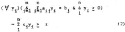
The algorithm can be used on formula (2), eliminating all the variables yi' l~i~n. The formula equivalent to (2), with z as the only variable, must express the same mathematical statement expressed in (2), namely that z is less than or equal to the minimum cost, c, if it exists. If no solution exists there are 2 possi bilities: The constraints may be inconsistent, or else they may include such values of yi so that the sum E ciyi is unbounded below. In the former case, formula (2) will reduce to TRUE and in the latter case to FALSE.
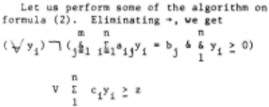
Changing universal quantifiers to existential quantifiers and eliminating negations we then get
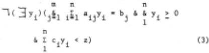
Formula (3) has the form: negation followed by a string of n existential quantifiers followed by a kernel consisting of a conjunction of m equalities and n+l inequalities. Allowing yi ~ 0 as an atom according to observation (2) above , we see that the kernel is trivially in disjunctive normal form as a pure conjunction. Also, when one quantifier, ( 3 yn) is eliminated
according to the modified algorithm, the result ing formula is still a pure conjunction. Thus, there is never any need to expand into disjunctive normal form, as each quantifier is eliminated in turn .
We give an example, which is given as an exer cise on the simplex algorithm in Gass (3).
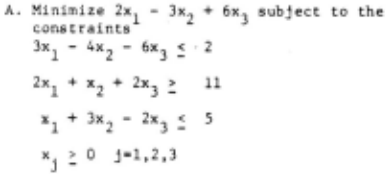
To set up this example for the simplex algo rith~, according to the reasonably standard version given in Gass, we convert A to the following equivalent problem.
- Minimize 2x 1 - 3x 2 + 6x 3 + wx 6 subject to the constraints
Here we require two slack variables, x 4 and x 7 , an excess variable, x 5 , and an auxiliary variable, x 6 · Also, the weight w in the object tive function, 2x 1 - 3x 2 + 6x 3 + wx 6 , must be larger than any fixed number so that x 6 will vanish in the so-called phase 1 of the simplex algorithm. We observe here that it is unnecess ary to go from statement A of the example to form B when using our algorithm to determine the minimum cost. Statement A can be used directly in formula (3) as follows:
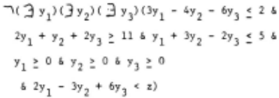
Note that the order of the three quantifiers is irrelevant so any of the variables y 1 ,y 2 ,y 3 can be eliminated first. We can therefore choose a yi that will lead to the minimum number of resulting atoms. We do this by counting the number of times each yi appears positively on either side of an inequality. We thus get Table 1.
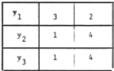
| yl | 3 | I 2 |
| Y2 | 1 | I 4 |
| y3 | 1 | I 4 I |
TABLE 1
We see that the choice of y 1 will yield 3x2=6 atoms from 3+2=5 atoms. Either y 2 or y 3 will yield only 4 atoms from 5 atoms. So, at least at the first elimination, the formula will expand less if we choose y 2 or y 3 .
Let us pick y 2 . The only inequality in which y 2 appears positively on the left is y 1 + 3y 2 - 2y 3 :: 5. We eliminate y 2 between this inequality and the others containing y 2 to obtain the new formula:
The same considerations as above lead to the choice of y 3 to be eliminated next:
or I ( z > 9 ) or z < 9. Therefore the minimum ·cost exists and is equal to 9.
We emphasize here that the linear programming example is used as a familiar problem for illus trative purposes. There are two drawbacks in using this method on typical linear programming problems.
- The formulation given above is used to determine the minimum cost but not the complete solution. Of course, the minimum cost can be used to verify an optimal solution or to deter mine exactly how far from optimal any feasible solution is.
- The main drawback is the lack of efficiency especially compared to the high efficiency of the simplex algorithm. The low efficiency of our algorithm is due to the expansion of the formula upon eliminating quantifiers.
Let us consider formula (3) above. The kernel is a conjunction of m equalities and n+l in equalities. As seen in Step 8 of the algorithm, when a quantifier is eliminated such that one of the conjuncts is an equality containing the quantified variable, there is no increase in the number of conjuncts. On the contrary there is a decrease of one. So, in general, m quantifiers can be eliminated using the equalities and re sulting in a formula with n-m quantifiers and n+l inequalities. Now each successive elimina tion of a quantifier from a formula with k in equalities can lead to a formula with (1)(1) · lLinequalities in the worst case, when 2 2 4
the occurrences on the left and right are bal anced. It appears that the worst case is also the most likely case and deviations of a few inequalities do not help much.
So, if n·B and m·4 then we could _end up with 1,562,500 inequalities. This seems the largest size that can be handled with this method in its present form.
We tried the algorithm on a dairy-feed diet problem due to Waugh (9) and presented in Gass (3). Here there were 10 variables and four inequalities; i.e., 10 feeds were combined to meet 4 minimum requirements at a minimum cost. The problem as initially stated proved too big for the program. How·ever, conversion to the dual problem; which had 4 variables and 14 inequalities, allowed de termination of the minimum cost. Even so, it took 12 hours on the PDP-10 under a LISP compiled version of the algorithm.
The use of a linear programming example, thus, is not to advocate use of this algorithm for linear programming, but to show that it can be used on practical problems.
The point we would like to emphasize t o skep tical readers is that although the EAR algorithm may not be efficient in given areas, its general ity allows application to various problems with no programs specific for each problem area.
For example, we can do non-linear programming whenever it is actually piecewise linear. Let us take the case of a piecewise linear objective function. These problems are not direct appli cations of the simplex algorithm. The optimal solutions may not even occur at the extreme points of the constraints. For example, suppose we wish to minimize the maximum of x 1 and x 2 under
Here, the optimum value of the objective function is 1/2 as opposed to a value of 1 at the .extreme points.
Piecewise linear functions can not only be ex pressed in terms of maximum and minimum as above, but also, equivalently, in terms of & and V. The above example can be stated in EAR as follows.
This is of course equivalent to z > 1/2 which can be verified by the algorithm.
General non-linear programming can also be approximated by using Chang (1). He shows how to do piecewise linear curve-fitting in n-dimensions. After using Chang's method to determine piecewise linear approximations, one can express the prob lem in EAR.
@inproceedings{ijcai1971p58,
  title     = {Solving Problems by Formula Manipulation in Logic and Linear Inequalities},
  author    = {Hodes, Louis},
  booktitle = {Proceedings of the Second International Joint Conference on
               Artificial Intelligence, {IJCAI-71}},
  publisher = {International Joint Conferences on Artificial Intelligence},
  editor    = {D.C. Cooper},
  pages     = {553--558},
  year      = {1971},
  url       = {https://ijcai.org/proceedings/1971/58},
}
TY - CPAPER TI - Solving Problems by Formula Manipulation in Logic and Linear Inequalities AU - Hodes, Louis T2 - Proceedings of the Second International Joint Conference on Artificial Intelligence, IJCAI-71 PB - International Joint Conferences on Artificial Intelligence PY - 1971 SP - 553 EP - 558 UR - https://ijcai.org/proceedings/1971/58 ER -Copied
Machine-readable versions of this paper, for tools and AI agents:
 Welcome
 Future Conferences
 AI Journal Division
 IJCAI Proceedings
 About IJCAI
 IJCAI Awards